This set of instructions will walk through how to setup an AWS S3 bucket for a specific project and how to configure that bucket to allow all members of the project team to have access.
Create an AWS account and S3 bucket
The first step is to create an AWS account that will be billed to your particular project. This can be done using these instructions.
Create AWS S3 bucket
Within your new AWS account, create an new S3 bucket:
- Open the AWS S3 console (https://
console .aws .amazon .com /s3 /) - From the navigation pane, choose Buckets
- Choose Create bucket
- Name the bucket and select us-west-2 for the region
- Leave all other default options
- Click Create Bucket
Create a user
Within the same AWS account, create a new IAM user:
- On the AWS Console Home page, select the IAM service
- In the navigation pane, select Users and then select Add users
- Name the user and click Next
- Attach policies directly
- Do not select any policies
- Click Next
- Create user
Once the user has been created, find the user’s ARN and copy it.
Now, create access keys for this user:
- Select Users and click the user that you created
- Open the Security Credentials tab
- Create access key
- Select Command Line Interface (CLI)
- Check the box to agree to the recommendation and click Next
- Leave the tag blank and click Create access key
- IMPORTANT: Copy the access key and the secret access key. This will be used later.
Create the bucket policy
Configure a policy for this S3 bucket that will allow the newly created user to access it.
- Open the AWS S3 console (https://
console .aws .amazon .com /s3 /) - From the navigation pane, choose Buckets
- Select the new S3 bucket that you created
- Open the Permissions tab
- Add the following bucket policy, replacing
USER_ARNwith the ARN that you copied above andBUCKET_ARNwith the bucket ARN, found on the Edit bucket policy page on the AWS console:
{
    "Version": "2012-10-17",
    "Statement": [
        {
            "Sid": "ListBucket",
            "Effect": "Allow",
            "Principal": {
                "AWS": "USER_ARN"
            },
            "Action": "s3:ListBucket",
            "Resource": "BUCKET_ARN"
        },
        {
            "Sid": "AllObjectActions",
            "Effect": "Allow",
            "Principal": {
                "AWS": "USER_ARN"
            },
            "Action": "s3:*Object",
            "Resource": "BUCKET_ARN/*"
        }
    ]
}
Configure local AWS profile
To access the bucket from a “local” computer (for example, a local computer or a JupyterHub that is running on AWS), an AWS profile must be configured with the access keys to the new S3 bucket.
This can be done manually but the easiest way to do it is by using AWS Command Line Interface (CLI).
On the local computer:
- Open a terminal
- Install AWS CLI (if using the
condapackage manager, you can install like this:conda install -c conda-forge awscli) - Configure the AWS profile with the keys from above and give your profile a new profile name:
aws configure --profile PROFILE_NAME- Enter the access key and secret access key
- Enter
us-west-2for the region andjsonfor format
In the code examples below, the profile name is icesat2. Replace this with the profile name that you used.
Example code
Below is code that can be used to read from and write to the S3 bucket in order to test that the bucket and local AWS profile have been configured correctly. Below each cell, there is expected output.
In the examples below, we are accessing a bucket called gris-outlet-glacier-seasonality-icesat2. Replace this name with the name of the S3 bucket that you have created.
Reading from the S3 bucket
Example: ls bucket using s3fs
import s3fs
s3 = s3fs.S3FileSystem(anon=False, profile='icesat2')
s3.ls('gris-outlet-glacier-seasonality-icesat2')
['gris-outlet-glacier-seasonality-icesat2/ATL06_20181020072141_03310105_001_01.h5',
 'gris-outlet-glacier-seasonality-icesat2/gsfc.glb_.200204_202104_rl06v1.0_sla-ice6gd.h5',
 'gris-outlet-glacier-seasonality-icesat2/new-file',
 'gris-outlet-glacier-seasonality-icesat2/out.tif',
 'gris-outlet-glacier-seasonality-icesat2/ssh_grids_v2205_1992101012.nc',
 'gris-outlet-glacier-seasonality-icesat2/temporary_test_file']
Example: open HDF5 file using xarray
import s3fs
import xarray as xr

fs_s3 = s3fs.core.S3FileSystem(profile='icesat2')

s3_url = 's3://gris-outlet-glacier-seasonality-icesat2/ssh_grids_v2205_1992101012.nc'
s3_file_obj = fs_s3.open(s3_url, mode='rb')
ssh_ds = xr.open_dataset(s3_file_obj, engine='h5netcdf')
print(ssh_ds)
<xarray.Dataset>
Dimensions:      (Longitude: 2160, nv: 2, Latitude: 960, Time: 1)
Coordinates:
  * Longitude    (Longitude) float32 0.08333 0.25 0.4167 ... 359.6 359.8 359.9
  * Latitude     (Latitude) float32 -79.92 -79.75 -79.58 ... 79.58 79.75 79.92
  * Time         (Time) datetime64[ns] 1992-10-10T12:00:00
Dimensions without coordinates: nv
Data variables:
    Lon_bounds   (Longitude, nv) float32 ...
    Lat_bounds   (Latitude, nv) float32 ...
    Time_bounds  (Time, nv) datetime64[ns] ...
    SLA          (Time, Latitude, Longitude) float32 ...
    SLA_ERR      (Time, Latitude, Longitude) float32 ...
Attributes: (12/21)
    Conventions:            CF-1.6
    ncei_template_version:  NCEI_NetCDF_Grid_Template_v2.0
    Institution:            Jet Propulsion Laboratory
    geospatial_lat_min:     -79.916664
    geospatial_lat_max:     79.916664
    geospatial_lon_min:     0.083333336
    ...                     ...
    version_number:         2205
    Data_Pnts_Each_Sat:     {"16": 661578, "1001": 636257}
    source_version:         commit dc95db885c920084614a41849ce5a7d417198ef3
    SLA_Global_MEAN:        -0.0015108844021796562
    SLA_Global_STD:         0.09098986023297456
    latency:                final
import s3fs

import xarray as xr

import hvplot.xarray
import holoviews as hv

fs_s3 = s3fs.core.S3FileSystem(profile='icesat2')

s3_url = 's3://gris-outlet-glacier-seasonality-icesat2/ssh_grids_v2205_1992101012.nc'
s3_file_obj = fs_s3.open(s3_url, mode='rb')
ssh_ds = xr.open_dataset(s3_file_obj, engine='h5netcdf')
ssh_da = ssh_ds.SLA

ssh_da.hvplot.image(x='Longitude', y='Latitude', cmap='Spectral_r', geo=True, tiles='ESRI', global_extent=True)
Example: read a geotiff using rasterio
import rasterio
import numpy as np
import matplotlib.pyplot as plt

session = rasterio.env.Env(profile_name='icesat2')

url = 's3://gris-outlet-glacier-seasonality-icesat2/out.tif'

with session:
    with rasterio.open(url) as ds:
        print(ds.profile)
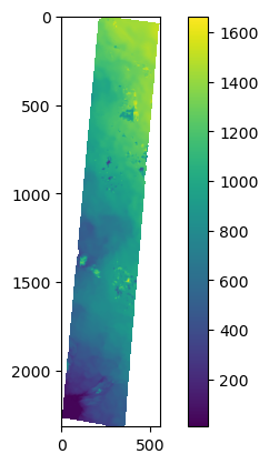
        band1 = ds.read(1)

band1[band1==-9999] = np.nan
plt.imshow(band1)
plt.colorbar()
{'driver': 'GTiff', 'dtype': 'float32', 'nodata': -9999.0, 'width': 556, 'height': 2316, 'count': 1, 'crs': CRS.from_epsg(3413), 'transform': Affine(50.0, 0.0, -204376.0,
       0.0, -50.0, -2065986.0), 'blockysize': 3, 'tiled': False, 'interleave': 'band'}

Writing to the S3 bucket
s3 = s3fs.core.S3FileSystem(profile='icesat2')

with s3.open('gris-outlet-glacier-seasonality-icesat2/new-file', 'wb') as f:
    f.write(2*2**20 * b'a')
    f.write(2*2**20 * b'a') # data is flushed and file closed

s3.du('gris-outlet-glacier-seasonality-icesat2/new-file')
4194304