Using ICESat-2 ATL15 (Gridded Arctic Land Ice Height) to investigate ice-surface height anomalies

Written by¶

Wilson Sauthoff (https://wsauthoff.github.io)
Luis Lopez (https://betolink.dev/)
Jessica Scheick (https://eos.unh.edu/person/jessica-scheick)
Tasha Snow (https://tsnow03.github.io)

Key learning outcomes:¶

How to gather data from disparate sources.
What is a Coordinate Reference System (CRS) and why it matters.
How to use geometries including Points and Polygons to define an area of interest and subset data.
The basics of how the icepyx library simplifies obtaining and interacting with ICESat-2 data.
How Xarray can simplify the import of multi-dimensional data.
Open, plot, and explore gridded raster data.

Computing environment¶

We will set up our computing environment with library imports and utility functions

Tip: If you need to import a library that is not pre-installed, use %pip install <package-name> alone within a Jupyter notebook cell to install it for this instance of CryoCloud (the pip installation will not presist between logins. All of the libraries we intend to use are pre-installed so we can skip this step.

%pip install icepyx==1.0.0

Requirement already satisfied: icepyx==1.0.0 in /srv/conda/envs/notebook/lib/python3.10/site-packages (1.0.0)
Requirement already satisfied: h5py in /srv/conda/envs/notebook/lib/python3.10/site-packages (from icepyx==1.0.0) (3.9.0)
Requirement already satisfied: fiona in /srv/conda/envs/notebook/lib/python3.10/site-packages (from icepyx==1.0.0) (1.9.4)
Requirement already satisfied: datashader in /srv/conda/envs/notebook/lib/python3.10/site-packages (from icepyx==1.0.0) (0.16.0)
Requirement already satisfied: shapely in /srv/conda/envs/notebook/lib/python3.10/site-packages (from icepyx==1.0.0) (2.0.1)
Requirement already satisfied: geopandas in /srv/conda/envs/notebook/lib/python3.10/site-packages (from icepyx==1.0.0) (0.13.2)
Requirement already satisfied: s3fs in /srv/conda/envs/notebook/lib/python3.10/site-packages (from icepyx==1.0.0) (2023.6.0)
Requirement already satisfied: xarray in /srv/conda/envs/notebook/lib/python3.10/site-packages (from icepyx==1.0.0) (2023.12.0)
Requirement already satisfied: earthaccess>=0.5.1 in /srv/conda/envs/notebook/lib/python3.10/site-packages (from icepyx==1.0.0) (0.8.2)
Requirement already satisfied: matplotlib in /srv/conda/envs/notebook/lib/python3.10/site-packages (from icepyx==1.0.0) (3.8.2)
Requirement already satisfied: requests in /srv/conda/envs/notebook/lib/python3.10/site-packages (from icepyx==1.0.0) (2.31.0)
Requirement already satisfied: holoviews in /srv/conda/envs/notebook/lib/python3.10/site-packages (from icepyx==1.0.0) (1.18.1)
Requirement already satisfied: numpy in /srv/conda/envs/notebook/lib/python3.10/site-packages (from icepyx==1.0.0) (1.23.5)
Requirement already satisfied: h5netcdf in /srv/conda/envs/notebook/lib/python3.10/site-packages (from icepyx==1.0.0) (1.1.0)
Requirement already satisfied: backoff in /srv/conda/envs/notebook/lib/python3.10/site-packages (from icepyx==1.0.0) (2.2.1)
Requirement already satisfied: hvplot in /srv/conda/envs/notebook/lib/python3.10/site-packages (from icepyx==1.0.0) (0.8.4)
Requirement already satisfied: tinynetrc<2.0.0,>=1.3.1 in /srv/conda/envs/notebook/lib/python3.10/site-packages (from earthaccess>=0.5.1->icepyx==1.0.0) (1.3.1)
Requirement already satisfied: pqdm>=0.1 in /srv/conda/envs/notebook/lib/python3.10/site-packages (from earthaccess>=0.5.1->icepyx==1.0.0) (0.2.0)
Requirement already satisfied: multimethod>=1.8 in /srv/conda/envs/notebook/lib/python3.10/site-packages (from earthaccess>=0.5.1->icepyx==1.0.0) (1.9.1)
Requirement already satisfied: python-dateutil>=2.8.2 in /srv/conda/envs/notebook/lib/python3.10/site-packages (from earthaccess>=0.5.1->icepyx==1.0.0) (2.8.2)
Requirement already satisfied: fsspec>=2022.11 in /srv/conda/envs/notebook/lib/python3.10/site-packages (from earthaccess>=0.5.1->icepyx==1.0.0) (2023.6.0)
Requirement already satisfied: python-cmr>=0.9.0 in /srv/conda/envs/notebook/lib/python3.10/site-packages (from earthaccess>=0.5.1->icepyx==1.0.0) (0.9.0)
Requirement already satisfied: certifi>=2017.4.17 in /srv/conda/envs/notebook/lib/python3.10/site-packages (from requests->icepyx==1.0.0) (2023.7.22)
Requirement already satisfied: urllib3<3,>=1.21.1 in /srv/conda/envs/notebook/lib/python3.10/site-packages (from requests->icepyx==1.0.0) (1.26.18)
Requirement already satisfied: idna<4,>=2.5 in /srv/conda/envs/notebook/lib/python3.10/site-packages (from requests->icepyx==1.0.0) (3.4)
Requirement already satisfied: charset-normalizer<4,>=2 in /srv/conda/envs/notebook/lib/python3.10/site-packages (from requests->icepyx==1.0.0) (3.3.0)
Requirement already satisfied: aiohttp!=4.0.0a0,!=4.0.0a1 in /srv/conda/envs/notebook/lib/python3.10/site-packages (from s3fs->icepyx==1.0.0) (3.9.1)
Requirement already satisfied: aiobotocore~=2.5.0 in /srv/conda/envs/notebook/lib/python3.10/site-packages (from s3fs->icepyx==1.0.0) (2.5.0)
Requirement already satisfied: numba in /srv/conda/envs/notebook/lib/python3.10/site-packages (from datashader->icepyx==1.0.0) (0.56.4)
Requirement already satisfied: pillow in /srv/conda/envs/notebook/lib/python3.10/site-packages (from datashader->icepyx==1.0.0) (9.5.0)
Requirement already satisfied: multipledispatch in /srv/conda/envs/notebook/lib/python3.10/site-packages (from datashader->icepyx==1.0.0) (0.6.0)
Requirement already satisfied: scipy in /srv/conda/envs/notebook/lib/python3.10/site-packages (from datashader->icepyx==1.0.0) (1.9.3)
Requirement already satisfied: colorcet in /srv/conda/envs/notebook/lib/python3.10/site-packages (from datashader->icepyx==1.0.0) (3.0.1)
Requirement already satisfied: toolz in /srv/conda/envs/notebook/lib/python3.10/site-packages (from datashader->icepyx==1.0.0) (0.12.0)
Requirement already satisfied: pyct in /srv/conda/envs/notebook/lib/python3.10/site-packages (from datashader->icepyx==1.0.0) (0.5.0)
Requirement already satisfied: dask in /srv/conda/envs/notebook/lib/python3.10/site-packages (from datashader->icepyx==1.0.0) (2022.11.0)
Requirement already satisfied: param in /srv/conda/envs/notebook/lib/python3.10/site-packages (from datashader->icepyx==1.0.0) (1.13.0)
Requirement already satisfied: pandas in /srv/conda/envs/notebook/lib/python3.10/site-packages (from datashader->icepyx==1.0.0) (1.5.1)
Requirement already satisfied: click~=8.0 in /srv/conda/envs/notebook/lib/python3.10/site-packages (from fiona->icepyx==1.0.0) (8.1.7)
Requirement already satisfied: cligj>=0.5 in /srv/conda/envs/notebook/lib/python3.10/site-packages (from fiona->icepyx==1.0.0) (0.7.2)
Requirement already satisfied: click-plugins>=1.0 in /srv/conda/envs/notebook/lib/python3.10/site-packages (from fiona->icepyx==1.0.0) (1.1.1)
Requirement already satisfied: six in /srv/conda/envs/notebook/lib/python3.10/site-packages (from fiona->icepyx==1.0.0) (1.16.0)
Requirement already satisfied: attrs>=19.2.0 in /srv/conda/envs/notebook/lib/python3.10/site-packages (from fiona->icepyx==1.0.0) (23.1.0)
Requirement already satisfied: packaging in /srv/conda/envs/notebook/lib/python3.10/site-packages (from geopandas->icepyx==1.0.0) (23.2)
Requirement already satisfied: pyproj>=3.0.1 in /srv/conda/envs/notebook/lib/python3.10/site-packages (from geopandas->icepyx==1.0.0) (3.6.1)
Requirement already satisfied: pyviz-comms>=0.7.4 in /srv/conda/envs/notebook/lib/python3.10/site-packages (from holoviews->icepyx==1.0.0) (2.3.2)
Requirement already satisfied: panel>=1.0 in /srv/conda/envs/notebook/lib/python3.10/site-packages (from holoviews->icepyx==1.0.0) (1.2.3)
Requirement already satisfied: bokeh>=1.0.0 in /srv/conda/envs/notebook/lib/python3.10/site-packages (from hvplot->icepyx==1.0.0) (3.2.2)
Requirement already satisfied: pyparsing>=2.3.1 in /srv/conda/envs/notebook/lib/python3.10/site-packages (from matplotlib->icepyx==1.0.0) (3.1.1)
Requirement already satisfied: contourpy>=1.0.1 in /srv/conda/envs/notebook/lib/python3.10/site-packages (from matplotlib->icepyx==1.0.0) (1.2.0)
Requirement already satisfied: cycler>=0.10 in /srv/conda/envs/notebook/lib/python3.10/site-packages (from matplotlib->icepyx==1.0.0) (0.12.1)
Requirement already satisfied: kiwisolver>=1.3.1 in /srv/conda/envs/notebook/lib/python3.10/site-packages (from matplotlib->icepyx==1.0.0) (1.4.5)
Requirement already satisfied: fonttools>=4.22.0 in /srv/conda/envs/notebook/lib/python3.10/site-packages (from matplotlib->icepyx==1.0.0) (4.46.0)
Requirement already satisfied: aioitertools>=0.5.1 in /srv/conda/envs/notebook/lib/python3.10/site-packages (from aiobotocore~=2.5.0->s3fs->icepyx==1.0.0) (0.11.0)
Requirement already satisfied: botocore<1.29.77,>=1.29.76 in /srv/conda/envs/notebook/lib/python3.10/site-packages (from aiobotocore~=2.5.0->s3fs->icepyx==1.0.0) (1.29.76)
Requirement already satisfied: wrapt>=1.10.10 in /srv/conda/envs/notebook/lib/python3.10/site-packages (from aiobotocore~=2.5.0->s3fs->icepyx==1.0.0) (1.16.0)
Requirement already satisfied: async-timeout<5.0,>=4.0 in /srv/conda/envs/notebook/lib/python3.10/site-packages (from aiohttp!=4.0.0a0,!=4.0.0a1->s3fs->icepyx==1.0.0) (4.0.3)
Requirement already satisfied: yarl<2.0,>=1.0 in /srv/conda/envs/notebook/lib/python3.10/site-packages (from aiohttp!=4.0.0a0,!=4.0.0a1->s3fs->icepyx==1.0.0) (1.9.3)
Requirement already satisfied: frozenlist>=1.1.1 in /srv/conda/envs/notebook/lib/python3.10/site-packages (from aiohttp!=4.0.0a0,!=4.0.0a1->s3fs->icepyx==1.0.0) (1.4.0)
Requirement already satisfied: aiosignal>=1.1.2 in /srv/conda/envs/notebook/lib/python3.10/site-packages (from aiohttp!=4.0.0a0,!=4.0.0a1->s3fs->icepyx==1.0.0) (1.3.1)
Requirement already satisfied: multidict<7.0,>=4.5 in /srv/conda/envs/notebook/lib/python3.10/site-packages (from aiohttp!=4.0.0a0,!=4.0.0a1->s3fs->icepyx==1.0.0) (6.0.4)
Requirement already satisfied: PyYAML>=3.10 in /srv/conda/envs/notebook/lib/python3.10/site-packages (from bokeh>=1.0.0->hvplot->icepyx==1.0.0) (5.4.1)
Requirement already satisfied: Jinja2>=2.9 in /srv/conda/envs/notebook/lib/python3.10/site-packages (from bokeh>=1.0.0->hvplot->icepyx==1.0.0) (3.1.2)
Requirement already satisfied: xyzservices>=2021.09.1 in /srv/conda/envs/notebook/lib/python3.10/site-packages (from bokeh>=1.0.0->hvplot->icepyx==1.0.0) (2023.10.1)
Requirement already satisfied: tornado>=5.1 in /srv/conda/envs/notebook/lib/python3.10/site-packages (from bokeh>=1.0.0->hvplot->icepyx==1.0.0) (6.1)
Requirement already satisfied: pytz>=2020.1 in /srv/conda/envs/notebook/lib/python3.10/site-packages (from pandas->datashader->icepyx==1.0.0) (2023.3.post1)
Requirement already satisfied: mdit-py-plugins in /srv/conda/envs/notebook/lib/python3.10/site-packages (from panel>=1.0->holoviews->icepyx==1.0.0) (0.4.0)
Requirement already satisfied: typing-extensions in /srv/conda/envs/notebook/lib/python3.10/site-packages (from panel>=1.0->holoviews->icepyx==1.0.0) (4.8.0)
Requirement already satisfied: tqdm>=4.48.0 in /srv/conda/envs/notebook/lib/python3.10/site-packages (from panel>=1.0->holoviews->icepyx==1.0.0) (4.64.1)
Requirement already satisfied: linkify-it-py in /srv/conda/envs/notebook/lib/python3.10/site-packages (from panel>=1.0->holoviews->icepyx==1.0.0) (2.0.0)
Requirement already satisfied: bleach in /srv/conda/envs/notebook/lib/python3.10/site-packages (from panel>=1.0->holoviews->icepyx==1.0.0) (6.1.0)
Requirement already satisfied: markdown-it-py in /srv/conda/envs/notebook/lib/python3.10/site-packages (from panel>=1.0->holoviews->icepyx==1.0.0) (2.2.0)
Requirement already satisfied: markdown in /srv/conda/envs/notebook/lib/python3.10/site-packages (from panel>=1.0->holoviews->icepyx==1.0.0) (3.5.1)
Requirement already satisfied: bounded-pool-executor in /srv/conda/envs/notebook/lib/python3.10/site-packages (from pqdm>=0.1->earthaccess>=0.5.1->icepyx==1.0.0) (0.0.3)
Requirement already satisfied: cloudpickle>=1.1.1 in /srv/conda/envs/notebook/lib/python3.10/site-packages (from dask->datashader->icepyx==1.0.0) (3.0.0)
Requirement already satisfied: partd>=0.3.10 in /srv/conda/envs/notebook/lib/python3.10/site-packages (from dask->datashader->icepyx==1.0.0) (1.4.1)
Requirement already satisfied: setuptools in /srv/conda/envs/notebook/lib/python3.10/site-packages (from numba->datashader->icepyx==1.0.0) (68.2.2)
Requirement already satisfied: llvmlite<0.40,>=0.39.0dev0 in /srv/conda/envs/notebook/lib/python3.10/site-packages (from numba->datashader->icepyx==1.0.0) (0.39.1)
Requirement already satisfied: jmespath<2.0.0,>=0.7.1 in /srv/conda/envs/notebook/lib/python3.10/site-packages (from botocore<1.29.77,>=1.29.76->aiobotocore~=2.5.0->s3fs->icepyx==1.0.0) (1.0.1)
Requirement already satisfied: MarkupSafe>=2.0 in /srv/conda/envs/notebook/lib/python3.10/site-packages (from Jinja2>=2.9->bokeh>=1.0.0->hvplot->icepyx==1.0.0) (2.1.3)
Requirement already satisfied: locket in /srv/conda/envs/notebook/lib/python3.10/site-packages (from partd>=0.3.10->dask->datashader->icepyx==1.0.0) (1.0.0)
Requirement already satisfied: webencodings in /srv/conda/envs/notebook/lib/python3.10/site-packages (from bleach->panel>=1.0->holoviews->icepyx==1.0.0) (0.5.1)
Requirement already satisfied: uc-micro-py in /srv/conda/envs/notebook/lib/python3.10/site-packages (from linkify-it-py->panel>=1.0->holoviews->icepyx==1.0.0) (1.0.1)
Requirement already satisfied: mdurl~=0.1 in /srv/conda/envs/notebook/lib/python3.10/site-packages (from markdown-it-py->panel>=1.0->holoviews->icepyx==1.0.0) (0.1.0)
Note: you may need to restart the kernel to use updated packages.

# Needed for pandas read_excel
%pip install openpyxl

Collecting openpyxl
  Downloading openpyxl-3.1.2-py2.py3-none-any.whl (249 kB)
     ━━━━━━━━━━━━━━━━━━━━━━━━━━━━━━━━━━━━━━━ 250.0/250.0 kB 2.9 MB/s eta 0:00:0000:0100:01
Collecting et-xmlfile
  Downloading et_xmlfile-1.1.0-py3-none-any.whl (4.7 kB)
Installing collected packages: et-xmlfile, openpyxl
Successfully installed et-xmlfile-1.1.0 openpyxl-3.1.2
Note: you may need to restart the kernel to use updated packages.

%matplotlib widget

# import internal libraries
import os

# import external libraries
import earthaccess
import geopandas as gpd
import h5py
import hvplot.xarray
import icepyx as ipx
# import matplotlib as mpl
# mpl.use('TkAgg') 

import matplotlib.colors as colors
import matplotlib.pyplot as plt
import matplotlib.ticker as ticker
from mpl_toolkits.axes_grid1 import make_axes_locatable
import numpy as np
import pandas as pd
from pyproj import CRS, Transformer
import rioxarray
import s3fs
import xarray as xr

# define utility function
def ll2ps(lon, lat):
    """
    Transform coordinates from geodetic coordinates (lon, lat)
    to Greenland (epsg:3413) coordinates (x, y)
    x, y = ll2ps(lon, lat)
    Inputs
    * lon, lat in decimal degrees (lon: W is negative; lat: S is negative)
    Outputs
    * x, y in [m]
    """
    crs_ll = CRS("EPSG:4326")
    crs_xy = CRS("EPSG:3413")
    ll_to_xy = Transformer.from_crs(crs_ll, crs_xy, always_xy = True)
    x, y = ll_to_xy.transform(lon, lat)
    return x, y

Greenland subglacial lakes¶

There are two classes of subglacial lakes: stable and active. Stable lakes have had a stable volume over the observational record whereas active episodically drain and fill. We can observe active subglacial lakes using ice-surface deformation time series.

In this tutorial, we will focus on Greenland where active subglacial lakes have been inferred from surface height changes.

Northern hemisphere subglacial lakes compiled in a global inventory by Livingstone and others (2020):

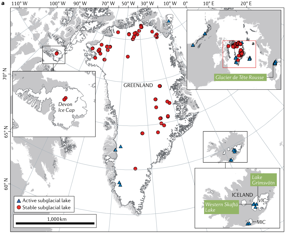
We can investigate active subglacial lakes using ice surface height anomalies as the overlying ice deforms when active lakes drain and fill episodically. These videos from NASA’s Science Visualization Studio illustrate how we observe active lakes filling and draining through time.

Locating the Greenland subglacial lakes¶

Consulting the supplementary data of the Livingstone and others (2020) inventory, we can construct a geopandas geodataframe to investigate Greenland’s subglacial lakes.

Opening non-cloud-hosted data uploaded to your CryoCloud Jupyter hub¶

If we are working with a dataset that is not cloud hosted or unavailable via a URL, we can upload that dataset to CryoCloud.

First, decide where the uploaded data will live on your CryoCloud hub. It could be a data directory folder that you create in your CryoCloud’s base directory or put the data into your working directory (whichever file management technique you prefer).

Second, download the paper’s supplementary data by clicking here.

Third, upload the supplementary data spreadsheet into your new data directory folder or your working directory. The supplementary data spreadsheet (.xlsx) is already uploaded to our working directory.

# Read in spreadsheet using pandas read_excel
use_cols = ['Name / Location', 'Lat. oN', 'Lon. oE', 'Lake Type', 'References']
import_rows = np.arange(0,65)
# You may add a path/to/file if you'd like to try reading spreadsheet from where you saved it in a data directory 
df = pd.read_excel('43017_2021_246_MOESM1_ESM.xlsx', 'Greenland', usecols=use_cols, skiprows = lambda x: x not in import_rows)

# View pandas dataset head (first 5 rows)
df.head()

However, since this data has a direct download URL, so we can read the data directly into CryoCloud skipping the download and upload steps, like so:

Open data directly via URL¶

# Read in spreadsheet using pandas read_excel
url = 'https://static-content.springer.com/esm/art%3A10.1038%2Fs43017-021-00246-9/MediaObjects/43017_2021_246_MOESM1_ESM.xlsx'
use_cols = ['Name / Location', 'Lat. oN', 'Lon. oE', 'Lake Type', 'References']
import_rows = np.arange(0,65)
df = pd.read_excel(url, sheet_name='Greenland', usecols=use_cols, skiprows = lambda x: x not in import_rows)

# View pandas dataset head (first 5 rows)
df.head()

This is looking good, but we can make it even better by storing the data in a GeoPandas GeoDataFrame which offers additional functionality beyond pandas. You can add a geometry column of Shapely objects that make geospatial data processing and visualization easier. Here we have Shapely points:

# Create GeoPandas GeoDataFrame from Pandas DataFrame
gdf = gpd.GeoDataFrame(
    df, geometry=gpd.points_from_xy(df['Lon. oE'], df['Lat. oN']))

# Set the Coordinate Reference System (CRS) of the geodataframe
if gdf.crs is None: 
    # set CRS WGS84 in lon, lat
    gdf.set_crs('epsg:4326', inplace=True)
    
# Display GeoDataFrame
gdf

Let’s look at Greenland’s active subglacial lake inventory by filtering on the Lake Type column:

# Let's look at Greenland's active subglacial lake inventory
gdf[gdf['Lake Type'] == 'Active']

Now let’s plot the lake locations to ensure our data read-in went as expected. But first, we need to make sure all projections for the data we want to show are the same.

What is a CRS/EPSG?¶

A Coordinate Reference System (CRS) tells you how the Earth’s 3-D surface is projected onto a 2-D plane map. Below are examples of various projections of continguous USA from an excellent Data Carpentry tutorial on the CRS topic:

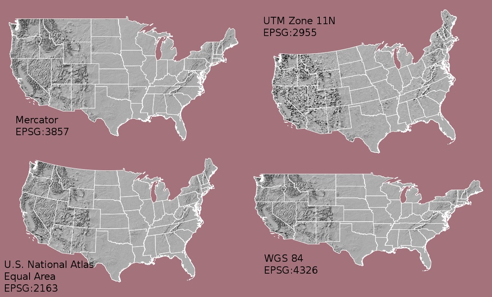
A particular CRS can be referenced by its EPSG code (e.g., epsg:4326 as we used in the GeoPandas GeoDataFrame example above). The EPSG is a structured dataset of CRS and Coordinate Transformations. It was originally compiled by the now defunct European Petroleum Survey Group (EPSG) but continues to be one common way of representing a specific CRS.
Most map projections make land areas look proportionally larger or smaller than they actually are. Below is intuitive visualization of this from another excellent site of tutorials on geospatial topics called Earth Lab:

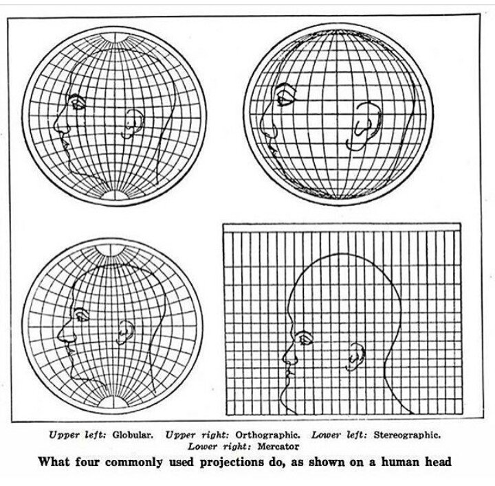
Because of this distortion, we select a projection that is best suited for the geographic region we are studying to minimize distortions.
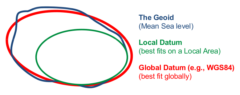
Previously we used epsg:4326, which is a geographic coordinate system that makes use of the World Geodetic System 1984 (WGS84) ellipsoid as a datum reference elevation. A datum consists in an ellipsoid relative to which the latitude and longitude of points are defined, with a geoid defining the surface at zero height (visual from ESA’s navipedia):

A geographic coordinate system is more than just the ellipsoid. It adds a coordinate system and units of measurement. epsg:4326 uses the very familiar longitude and latitude and degrees as the coordinate system and units. We selected epsg:4326 because longitude and latitude were the coordinates in the dataset.
There are numerous formats that are used to document a CRS. Three common formats include: proj.4, EPSG, and Well-known Text (WKT) formats.
Useful websites to look up CRS strings are spatialreference.org and espg.io. You can use the search on these sites to find an EPSG code.
Often you have data in one format or projection (CRS) and you need to transform it to a more regionally accurate CRS or match it to another datasets’ CRS to plot them together. Let’s transform our geopandas data to the NSIDC Sea Ice North Polar Stereographic projection (epsg:3413) easily visualize our lakes on a projection that minimizes distortion of our area of interest (Greenland).

# Load "Natural Earth” countries dataset, bundled with GeoPandas
world = gpd.read_file(gpd.datasets.get_path('naturalearth_lowres'))
Greenland = world[world['name'] == 'Greenland']

# Create a rough plot to ensure data was read properly
fig, axs = plt.subplots(1,2, figsize=(7,6.5))
Greenland.plot(ax=axs[0], facecolor='lightgray', edgecolor='gray')
gdf[gdf['Lake Type'] == 'Active'].plot(ax=axs[0], label='active subglacial lake')
axs[0].set_xlabel('northing (m)'); axs[0].set_ylabel('easting (m)')
axs[0].set_title('epsg:4326: WGS84\nWorld Geodetic System 1984')
axs[0].legend()
             
Greenland.to_crs('epsg:3413').plot(ax=axs[1], facecolor='lightgray', edgecolor='gray')
gdf[gdf['Lake Type'] == 'Active'].to_crs('epsg:3413').plot(ax=axs[1], label='active subglacial lake')
axs[1].set_xlabel('northing (m)'); axs[1].set_ylabel('easting (m)')
axs[1].set_title('epsg:3413: WGS84 / NSIDC \nSea Ice Polar Stereographic North')
axs[1].legend()
fig.suptitle('Active subglacial lake distribution\nacross Greenland in two projections')
plt.show()

Using the Shapely Polygon geometry to create a search radius and subset data¶

The Shapely points used before are useful to tell us the centroid of the lakes.
However, we’d like to be able to create a search radius around that point to search for and subset data.
Some datasets are massive, so using Shapely polygons as a search radius around your region of interest will speed up your computation.

# Create GeoSeries of our GeoDataFrame that converts to Arcic polar stereographic projection 
# and makes 10-km radius buffered polygon around each lake point
gs = gdf.to_crs('3413').buffer(10000)

# Create a copy of the original GeoPandas GeoDataFrame so that we don't alter the original
gdf_polys = gdf.copy(deep=True)

# Create new GeoDataFrame to store the polygons
gdf_polys = gpd.GeoDataFrame(gdf, 
                             # We use the GeoDataFrame (gdf) copy, gdf_polys, and replaced its geometry with the GeoSeries of polygons
                             geometry=gs, 
                             # We must specify the crs, so we use the one used to create the GeoSeries of polygons
                             crs='epsg:3413'
                             # But then we switch the crs back to good ol' 4623 lon, lat
                             ).to_crs('4623')

# Look at active lakes to ensure it worked as expected
gdf_polys[gdf_polys['Lake Type'] == 'Active']

Now that we know our active lake locations, let’s grab data to study the filling and draining of the lakes. We will use ICESat-2 surface elevations to investigate.

What is ICESat-2?¶

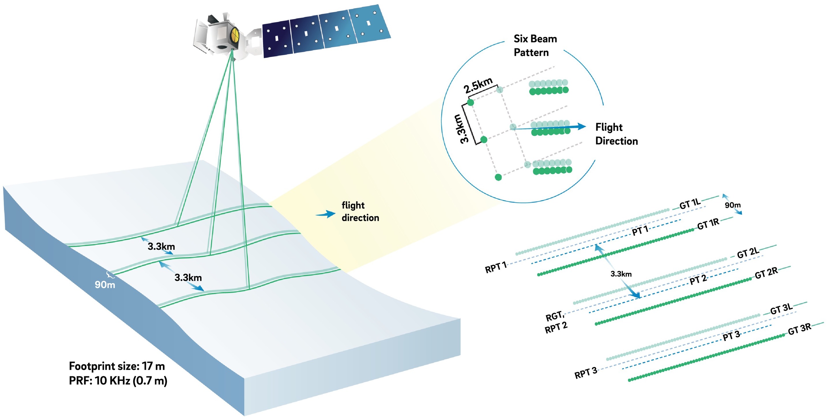
ICESat-2 (Ice, Cloud, and land Elevation Satellite 2), part of NASA’s Earth Observing System, is a satellite mission for measuring ice sheet elevation and sea ice thickness, as well as land topography, vegetation characteristics, and clouds. It does so using an altimeter or an altitude meter, which is an instrument used to measure the altitude of an object above a fixed level (the datum we talked about earlier). This is typically achieved by measuring the time it takes for a lidar or radar pulse, released by a satellite-based altimeter, to travel to a surface, reflect, and return to be recorded by an onboard instrument. ICESat-2 uses three pairs of laser pulsers and the detector to count the reflected photons.

ICESat-2 laser configuration (from Smith and others, 2019):

What is ATL14/15?¶

ATL15 is one of the various ICESat-2 data products. ATL15 provides various resolutions (1 km, 10 km, 20 km, and 40 km) of gridded raster data of height change at 3-month intervals, allowing for visualization of height-change patterns and calculation of integrated active subglacial lake volume change (Smith and others, 2022).

ATL14 is an accompnaying high-resolution (100 m) digital elevation model (DEM) that provides spatially continuous gridded data of ice sheet surface height.

Learn more about the ICESat-2 ATL14/15 Gridded Antarctic and Arctic Land Ice Height Change data product dataset here.

Streaming cloud-hosted data from NASA Earth Data Cloud¶

We will be working with cloud-hosted data files. This guide explains how to find and access Earthdata cloud-hosted data. Here is a complete list of earthdata cloud-hosted data products currently available from NSIDC.

Using icepyx to simplify searching for ICESat-2 data¶

icepyx is a community and Python software library that simplifies the process of searching (querying), accessing (via download or in the cloud), and working with (including subsetting, visualizing, and reading in) ICESat-2 data products. A series of examples introduce users to its functionality, and the icepyx community always welcomes new members, feature requests, bug reports, etc.

To search for data spatially, icepyx accepts shapefiles, kml files, and geopackage files, as well as bounding boxes and polygons, as input bounding regions. So we’ll first save one of the lakes’ geometries as a geopackage and use it to query ICESat-2 data for that region.

# Export to geopackage to subset ICESat-2 data
gdf_polys[gdf_polys['Name / Location'] == 'Flade Isblink ice cap'].to_file(os.getcwd() + '/Flade_Isblink_poly.gpkg')

# Specifying the necessary icepyx parameters
short_name = 'ATL15'  # The data product we would like to query
spatial_extent = 'Flade_Isblink_poly.gpkg'
date_range = ['2018-09-15','2023-03-02']

# Setup the Query object
region = ipx.Query(short_name, spatial_extent, date_range)

We can visualize our spatial extent on an interactive map with background imagery.

# Visualize area of interest
region.visualize_spatial_extent()

# Let's find out some information about the available data granuales (files)
region.avail_granules()

{'Number of available granules': 4,
 'Average size of granules (MB)': 193.56415557861328,
 'Total size of all granules (MB)': 774.2566223144531}

ipx.__version__

'1.0.0'

# Let's see the granule IDs and cloud access urls
gran_ids = region.avail_granules(ids=True, cloud=True)
gran_ids
s3url='s3://nsidc-cumulus-prod-protected/ATLAS/ATL15/002/2019/ATL15_GL_0314_01km_002_01.nc'

# Let's grab the s3 URL of the highest resolution available product
s3url = gran_ids[1][3]
s3url

's3://nsidc-cumulus-prod-protected/ATLAS/ATL15/002/2019/ATL15_GL_0314_01km_002_01.nc'

You can manually find s3 URL’s for cloud-hosted data from NASA Earth Data

Learn more about finding cloud-hosted data from NASA Earth data cloud here

The next step (accessing data in the cloud) requires a NASA Earthdata user account. You can register for a free account here. icepyx will automatically ask for your credentials when you perform a task that needs them. If you do not have them stored as environment variables or in a .netrc file, you will be prompted to enter them.

# set up our s3 file system using our credentials
s3 = earthaccess.get_s3fs_session(daac='NSIDC', provider=region._s3login_credentials)

# Open s3url data file and store in Xarray Dataset
# This cell takes 10s of secs to load
with s3.open(s3url,'rb') as f:
    # ATL15_dh = rioxarray.open_rasterio(f, group='delta_h').load()  # FIXME: preferred, but giving error
    ATL15_dh = xr.open_dataset(f, group='delta_h').load()

# View Xarray Dataset
ATL15_dh

reader = ipx.Read(s3url)

Enter your Earthdata Login username:  icepyx_devteam
Enter your Earthdata password:  ········

# Indicate which variables you'd like to read in.
# More information on managing ICESat-2 variables is available in the icepyx documentation and examples.
reader.vars.append(var_list=["delta_h"])

---------------------------------------------------------------------------
ValueError                                Traceback (most recent call last)
Cell In [22], line 1
----> 1 reader.vars.append(var_list=["delta_h"])

File /srv/conda/envs/notebook/lib/python3.10/site-packages/icepyx/core/variables.py:496, in Variables.append(self, defaults, var_list, beam_list, keyword_list)
    487 assert not (
    488     defaults == False
    489     and var_list == None
    490     and beam_list == None
    491     and keyword_list == None
    492 ), "You must enter parameters to add to a variable subset list. If you do not want to subset by variable, ensure your is2.subsetparams dictionary does not contain the key 'Coverage'."
    494 final_vars = {}
--> 496 vgrp, allpaths = self.avail(options=True, internal=True)
    497 self._check_valid_lists(vgrp, allpaths, var_list, beam_list, keyword_list)
    499 # Instantiate self.wanted to an empty dictionary if it doesn't exist

File /srv/conda/envs/notebook/lib/python3.10/site-packages/icepyx/core/variables.py:150, in Variables.avail(self, options, internal)
    148 if not hasattr(self, "_avail") or self._avail == None:
    149     if not hasattr(self, "path") or self.path.startswith("s3"):
--> 150         self._avail = is2ref._get_custom_options(
    151             self.session, self.product, self.version
    152         )["variables"]
    153     else:
    154         # If a path was given, use that file to read the variables
    155         import h5py

File /srv/conda/envs/notebook/lib/python3.10/site-packages/icepyx/core/is2ref.py:112, in _get_custom_options(session, product, version)
    110 format_vals = [formats[i]["value"] for i in range(len(formats))]
    111 try:
--> 112     format_vals.remove("")
    113 except KeyError:
    114     # ATL23 does not have an empty value
    115     pass

ValueError: list.remove(x): x not in list

We can acquaint ourselves with this dataset in a few ways:

The data product’s overview page (Smith and others, 2022) to get the very basics such as geographic coverage, CRS, and what the data product tells us (quarterly height changes).
The Xarray Dataset read-in metadata: clicking on the written document icon of each data variable will expand metadata including a data variable’s dimensions, datatype, etc.
The data product’s data dictionary (Smith and others, 2021) to do a deep dive on what individual variables tell us.
THe data product’s Algorithm Theoretical Basis Document

We’ll be plotting the delta_h data variable in this tutorial, here’s what we can learn about from these sources:

ATL14/15’s overview page: this is likely the ‘quarterly height changes’ described, but let’s dive deeper to be sure
ATL14/15’s Xarray Dataset imbedded metadata tells us a couple things: delta_h =height change at 1 km (the resolution selected earlier) and height change relative to the datum (Jan 1, 2020) surface
ATL14/15’s data dictionary: delta_h = quarterly height change at 40 km

Ok, since the data is relative to a datum, we have two options:

Difference individual time slices to subtract out the datum, like so:
(time₀ - datum) - (time₁ - datum) = time₀ - datum - time₁ + datum = time₀ - time₁
Subtract out the datum directly. The datum is the complementary dataset high-resolution DEM surface contained in tha accompanying dataset ATL14.

In this tutorial we’ll use the first method. We’ll use some explanatory data analysis to illustrate this.

# Let's make a simple plot of the first minus the zeroth time slices
fig, ax = plt.subplots(figsize=(6,3))
dhdt = ATL15_dh['delta_h'][1,:,:] - ATL15_dh['delta_h'][0,:,:]
cb = ax.imshow(dhdt, origin='lower', norm=colors.CenteredNorm(), cmap='coolwarm_r', 
               extent=[Greenland.bounds.minx.values[0], Greenland.bounds.maxx.values[0], Greenland.bounds.miny.values[0], Greenland.bounds.maxy.values[0]])
ax.set_xlabel('longitude'); ax.set_ylabel('latitude')
plt.colorbar(cb, fraction=0.02, label='height change [m]')
plt.show()

Hmmm...doesn’t look like much change over this quarter. Why? Check out the bounds of the colorbar, we’ve got some pretty extreme values (colorbar is defaulting to ±10 m!) that appear to be along the margin. It’s making more sense now. We can change the bounds of the colorbar to plot see more of the smaller scale change in the continental interior.

# Let's calculate some basic stats to determine appropriate coloarbar bounds
print(dhdt.min().values)
print(dhdt.max().values)

-3.6538086
10.285828

We can use a TwoSlopeNorm to achieve different mapping for positive and negative values while still keeping the center at zero:

# We can make that same plot with more representative colorbar bounds
fig, ax = plt.subplots(figsize=(6,3))
dhdt = ATL15_dh['delta_h'][1,:,:] - ATL15_dh['delta_h'][0,:,:]
divnorm = colors.TwoSlopeNorm(vmin=dhdt.min(), vcenter=0, vmax=dhdt.max())
cb = ax.imshow(dhdt, origin='lower', norm=divnorm, cmap='coolwarm_r', 
               extent=[Greenland.bounds.minx.values[0], Greenland.bounds.maxx.values[0], Greenland.bounds.miny.values[0], Greenland.bounds.maxy.values[0]])
ax.set_xlabel('longitude'); ax.set_ylabel('latitude')
plt.colorbar(cb, fraction=0.02, label='height change [m]')
plt.show()

Now the colorbar bounds are more representative, but we still have the issue that extreme values along the margin are swapping any signals we might see in the continental interior.

# Let's use the Xarray DataArray quantile method to find the 1% and 99% quantiles (Q1 and Q3) of the data
dhdt.quantile([0.01,0.99])

We can use these quantiles as the colorbar bounds so that we see the data variability by plotting the most extreme values at the maxed out value of the colorbar. We’ll adjust the caps of the colorbar (using extend) to express that there are data values beyond the bounds.

# Let's make the same plot but using the quantiles as the colorbar bounds
fig, ax = plt.subplots(figsize=(6,3))
dhdt = ATL15_dh['delta_h'][1,:,:] - ATL15_dh['delta_h'][0,:,:]
divnorm = colors.TwoSlopeNorm(vmin=dhdt.quantile(0.01), vcenter=0, vmax=dhdt.quantile(0.99))
cb = ax.imshow(dhdt, origin='lower', norm=divnorm, cmap='coolwarm_r', 
               extent=[Greenland.bounds.minx.values[0], Greenland.bounds.maxx.values[0], Greenland.bounds.miny.values[0], Greenland.bounds.maxy.values[0]])
ax.set_xlabel('longitude'); ax.set_ylabel('latitude')
plt.colorbar(cb, fraction=0.02, extend='both', label='height change [m]')
plt.tight_layout()
plt.show()

# Let's make the same plot but for all the available time slices and let's turn it in a function so that we can reuse this code for a smaller subset of data
# create empty lists to store data
def plot_icesat2_atl15(xmin, xmax, ymin, ymax, dataset):
    # subset data using bounding box in epsg:3134 x,y
    mask_x = (dataset.x >= xmin) & (dataset.x <= xmax)
    mask_y = (dataset.y >= ymin) & (dataset.y <= ymax)
    ds_sub = dataset.where(mask_x & mask_y, drop=True)
    
    # Create empty lists to store data
    vmins_maxs = []

    # Find the min's and max's of each inter time slice comparison and store into lists
    for idx in range(len(ds_sub['time'].values)-1): 
        dhdt = ds_sub['delta_h'][idx+1,:,:] - ds_sub['delta_h'][idx,:,:]
        vmin=dhdt.quantile(0.01)
        vmins_maxs += [vmin]
        vmax=dhdt.quantile(0.99)
        vmins_maxs += [vmax]
        if (min(vmins_maxs)<0) & (max(vmins_maxs)>0):
            vcenter = 0
        else: 
            vcenter = max(vmins_maxs) - min(vmins_maxs)
        divnorm = colors.TwoSlopeNorm(vmin=min(vmins_maxs), vcenter=vcenter, vmax=max(vmins_maxs))

    # create fig, ax
    fig, axs = plt.subplots(7,2, sharex=True, sharey=True, figsize=(10,10))

    idx = 0
    for ax in axs.ravel():   
        ax.set_aspect('equal')
        dhdt = ds_sub['delta_h'][idx+1,:,:] - ds_sub['delta_h'][idx,:,:]
        cb = ax.imshow(dhdt, origin='lower', norm=divnorm, cmap='coolwarm_r', 
                       extent=[xmin[0], xmax[0], ymin[0], ymax[0]])
        # Change polar stereographic m to km
        km_scale = 1e3
        ticks_x = ticker.FuncFormatter(lambda x, pos: '{0:g}'.format(x/km_scale))
        ax.xaxis.set_major_formatter(ticks_x)
        ticks_y = ticker.FuncFormatter(lambda x, pos: '{0:g}'.format(x/km_scale))
        ax.yaxis.set_major_formatter(ticks_y)
        # Create common axes labels
        fig.supxlabel('easting (km)'); fig.supylabel('northing (km)')
        # Increment the idx
        idx = idx + 1
     
    fig.colorbar(cb, extend='both', ax=axs.ravel().tolist(), label='height change [m]')
    plt.show()

Let’s zoom into an individual active lake to see more detail. First let’s remind ourselves of the Greenland active subglacial lakes by filtering on lake type:

gdf_polys_active = gdf_polys[gdf_polys['Lake Type'] == 'Active']
gdf_polys_active

# We can call the bounds of the geometry of the Shapely Polygon we created earlier
gdf_sub = gdf_polys_active[gdf_polys_active['Name / Location'] == 'Inuppaat Quuat']

Now using these geometry bounds we can plot the area immediately around the active subglacial lake.

# If the figure doesn't pop up, it is because the holoviews plot was run immediately after and interferred with 
# matplotlib. Just rerun this cell and it will be fixed
%matplotlib widget

# Assigning the min, max lon, lat coords of the lower-left and upper-right corners of our bounding box 
# around the lake's buffer polygon
lon_min = gdf_sub.geometry.bounds.minx
lon_max = gdf_sub.geometry.bounds.maxx
lat_min = gdf_sub.geometry.bounds.miny
lat_max = gdf_sub.geometry.bounds.maxy

# Now we re-project the lon, lat into x, y coords in the 3413 CRS, which ATL15 uses
xmin, ymin = ll2ps(lon_min, lat_min)
xmax, ymax = ll2ps(lon_max, lat_max)

# Use our plotting fuction to plot up the data based on min, max x, y bounds
plot_icesat2_atl15(xmin, xmax, ymin, ymax, ATL15_dh)

# Let's explore plotting the data interactively using Xarray and Holoviews
hvplot.extension('matplotlib')
divnorm = colors.TwoSlopeNorm(vmin=-0.25, vcenter=0, vmax=1.25)
ATL15_dh['delta_h'].hvplot(groupby='time', cmap='coolwarm_r', norm=divnorm, invert=True, 
                           width=(ATL15_dh['x'].max()-ATL15_dh['x'].min())/3e3, height=(ATL15_dh['y'].max()-ATL15_dh['y'].min())/3e3, 
                           widget_type='scrubber', widget_location='bottom')

# clean up environment by deleting intermediary files
os.remove('Flade_Isblink_poly.gpkg')

Streaming cloud-hosted data via earthaccess¶

We will next use earthaccess to authenicate for NASA EarthData, and search and stream cloud-hosted data directly.

# Import earthaccess Library and view version
import earthaccess
print(f"Using earthaccess v{earthaccess.__version__}")

Using earthaccess v0.5.3

Log into NASA’s Earthdata using the earthaccess package¶

There are multiple ways to provide your Earthdata credentials via earthaccess. The earthaccess authentication class automatically tries three methods for getting user credentials to log in:

with EARTHDATA_USERNAME and EARTHDATA_PASSWORD environment variables
through an interactive, in-notebook login (used below); passwords are not shown plain text
with stored credentials in a .netrc file (not recommended for security reasons)

# Try to authenticate
auth = earthaccess.login()
print(auth.authenticated)

We are already authenticated with NASA EDL
True

Search for cloud-available datasets from NASA¶

# Using a keyword search

from pprint import pprint
datasets = earthaccess.search_datasets(keyword="SENTINEL",
                                       cloud_hosted=True)

for dataset in datasets[0:2]:
    pprint(dataset.summary())

Datasets found: 131
{'concept-id': 'C1595422627-ASF',
 'file-type': '',
 'get-data': [],
 'short-name': 'SENTINEL-1_INTERFEROGRAMS',
 'version': '1'}
{'cloud-info': {'Region': 'us-west-2',
                'S3BucketAndObjectPrefixNames': ['s3://lp-prod-protected/HLSS30.020',
                                                 's3://lp-prod-public/HLSS30.020'],
                'S3CredentialsAPIDocumentationURL': 'https://data.lpdaac.earthdatacloud.nasa.gov/s3credentialsREADME',
                'S3CredentialsAPIEndpoint': 'https://data.lpdaac.earthdatacloud.nasa.gov/s3credentials'},
 'concept-id': 'C2021957295-LPCLOUD',
 'file-type': "[{'Format': 'Cloud Optimized GeoTIFF (COG)', 'FormatType': "
              "'Native', 'Media': ['Earthdata Cloud', 'HTTPS'], "
              "'AverageFileSize': 20.0, 'AverageFileSizeUnit': 'MB', "
              "'TotalCollectionFileSizeBeginDate': "
              "'2015-11-28T00:00:00.000Z'}]",
 'get-data': ['https://search.earthdata.nasa.gov/search?q=C2021957295-LPCLOUD',
              'https://appeears.earthdatacloud.nasa.gov/'],
 'short-name': 'HLSS30',
 'version': '2.0'}

# Using a known short name
datasets = earthaccess.search_datasets(short_name="HLSS30",
                                       cloud_hosted=True)
for dataset in datasets:
    pprint(dataset.summary())
    pprint(dataset.abstract())

Datasets found: 1
{'cloud-info': {'Region': 'us-west-2',
                'S3BucketAndObjectPrefixNames': ['s3://lp-prod-protected/HLSS30.020',
                                                 's3://lp-prod-public/HLSS30.020'],
                'S3CredentialsAPIDocumentationURL': 'https://data.lpdaac.earthdatacloud.nasa.gov/s3credentialsREADME',
                'S3CredentialsAPIEndpoint': 'https://data.lpdaac.earthdatacloud.nasa.gov/s3credentials'},
 'concept-id': 'C2021957295-LPCLOUD',
 'file-type': "[{'Format': 'Cloud Optimized GeoTIFF (COG)', 'FormatType': "
              "'Native', 'Media': ['Earthdata Cloud', 'HTTPS'], "
              "'AverageFileSize': 20.0, 'AverageFileSizeUnit': 'MB', "
              "'TotalCollectionFileSizeBeginDate': "
              "'2015-11-28T00:00:00.000Z'}]",
 'get-data': ['https://search.earthdata.nasa.gov/search?q=C2021957295-LPCLOUD',
              'https://appeears.earthdatacloud.nasa.gov/'],
 'short-name': 'HLSS30',
 'version': '2.0'}
('The Harmonized Landsat Sentinel-2 (HLS) project provides consistent surface '
 'reflectance data from the Operational Land Imager (OLI) aboard the joint '
 'NASA/USGS Landsat 8 satellite and the Multi-Spectral Instrument (MSI) aboard '
 'Europe’s Copernicus Sentinel-2A and Sentinel-2B satellites. The combined '
 'measurement enables global observations of the land every 2–3 days at '
 '30-meter (m) spatial resolution. The HLS project uses a set of algorithms to '
 'obtain seamless products from OLI and MSI that include atmospheric '
 'correction, cloud and cloud-shadow masking, spatial co-registration and '
 'common gridding, illumination and view angle normalization, and spectral '
 'bandpass adjustment. \r\n'
 '\r\n'
 'The HLSS30 product provides 30-m Nadir Bidirectional Reflectance '
 'Distribution Function (BRDF)-Adjusted Reflectance (NBAR) and is derived from '
 'Sentinel-2A and Sentinel-2B MSI data products. The HLSS30 and HLSL30 '
 'products are gridded to the same resolution and Military Grid Reference '
 'System (MGRS) '
 '(https://hls.gsfc.nasa.gov/products-description/tiling-system/) tiling '
 'system, and thus are “stackable” for time series analysis.\r\n'
 '\r\n'
 'The HLSS30 product is provided in Cloud Optimized GeoTIFF (COG) format, and '
 'each band is distributed as a separate COG. There are 13 bands included in '
 'the HLSS30 product along with four angle bands and a quality assessment (QA) '
 'band. See the User Guide for a more detailed description of the individual '
 'bands provided in the HLSS30 product.\r\n')

Searching for granules (files) from a given collection (dataset)¶

earthaccess has two different ways of querying for data:

We can build a query object or
we can use the top level API.

The difference is that the query object is a bit more flexible and we don’t retrieve the metadata from CMR until we execute the .get() or .get_all() methods.

Let’s use bboxfinder.com to get the extent of our bounding box and enter it into our bounding box input below. You are also welcome to put in a bounding box you already have available. You can uncomment the Iceland bounding box if you don’t want to find your own. Order should be: min_lon, min_lat, max_lon, max_lat

# Using a specific concept-id, which is unique to the specific product and version

# bbox for ~Iceland is -22.1649, 63.3052, -11.9366, 65.5970 
granules_query = earthaccess.granule_query().cloud_hosted(True) \
        .concept_id("C2021957295-LPCLOUD") \
        .bounding_box(-22.1649, 63.3052, -11.9366, 65.5970) \
        .temporal("2020-01-01","2023-01-01")
granules_query.params

{'concept_id': ['C2021957295-LPCLOUD'],
 'bounding_box': '-22.1649,63.3052,-11.9366,65.597',
 'temporal': ['2020-01-01T00:00:00Z,2023-01-01T00:00:00Z']}

granules_query.hits()

5380

Earthaccess has many methods we can use for our search. For a complete list of the parameters we can use, go to https://nsidc.github.io/earthaccess/user-reference/granules/granules-query/

granule = granules_query.get(1)[0]
granule.data_links()

['https://data.lpdaac.earthdatacloud.nasa.gov/lp-prod-protected/HLSS30.020/HLS.S30.T27VWL.2020048T131259.v2.0/HLS.S30.T27VWL.2020048T131259.v2.0.B09.tif',
 'https://data.lpdaac.earthdatacloud.nasa.gov/lp-prod-protected/HLSS30.020/HLS.S30.T27VWL.2020048T131259.v2.0/HLS.S30.T27VWL.2020048T131259.v2.0.B05.tif',
 'https://data.lpdaac.earthdatacloud.nasa.gov/lp-prod-protected/HLSS30.020/HLS.S30.T27VWL.2020048T131259.v2.0/HLS.S30.T27VWL.2020048T131259.v2.0.B10.tif',
 'https://data.lpdaac.earthdatacloud.nasa.gov/lp-prod-protected/HLSS30.020/HLS.S30.T27VWL.2020048T131259.v2.0/HLS.S30.T27VWL.2020048T131259.v2.0.B03.tif',
 'https://data.lpdaac.earthdatacloud.nasa.gov/lp-prod-protected/HLSS30.020/HLS.S30.T27VWL.2020048T131259.v2.0/HLS.S30.T27VWL.2020048T131259.v2.0.B08.tif',
 'https://data.lpdaac.earthdatacloud.nasa.gov/lp-prod-protected/HLSS30.020/HLS.S30.T27VWL.2020048T131259.v2.0/HLS.S30.T27VWL.2020048T131259.v2.0.B06.tif',
 'https://data.lpdaac.earthdatacloud.nasa.gov/lp-prod-protected/HLSS30.020/HLS.S30.T27VWL.2020048T131259.v2.0/HLS.S30.T27VWL.2020048T131259.v2.0.B07.tif',
 'https://data.lpdaac.earthdatacloud.nasa.gov/lp-prod-protected/HLSS30.020/HLS.S30.T27VWL.2020048T131259.v2.0/HLS.S30.T27VWL.2020048T131259.v2.0.Fmask.tif',
 'https://data.lpdaac.earthdatacloud.nasa.gov/lp-prod-protected/HLSS30.020/HLS.S30.T27VWL.2020048T131259.v2.0/HLS.S30.T27VWL.2020048T131259.v2.0.B8A.tif',
 'https://data.lpdaac.earthdatacloud.nasa.gov/lp-prod-protected/HLSS30.020/HLS.S30.T27VWL.2020048T131259.v2.0/HLS.S30.T27VWL.2020048T131259.v2.0.SAA.tif',
 'https://data.lpdaac.earthdatacloud.nasa.gov/lp-prod-protected/HLSS30.020/HLS.S30.T27VWL.2020048T131259.v2.0/HLS.S30.T27VWL.2020048T131259.v2.0.VAA.tif',
 'https://data.lpdaac.earthdatacloud.nasa.gov/lp-prod-protected/HLSS30.020/HLS.S30.T27VWL.2020048T131259.v2.0/HLS.S30.T27VWL.2020048T131259.v2.0.SZA.tif',
 'https://data.lpdaac.earthdatacloud.nasa.gov/lp-prod-protected/HLSS30.020/HLS.S30.T27VWL.2020048T131259.v2.0/HLS.S30.T27VWL.2020048T131259.v2.0.B02.tif',
 'https://data.lpdaac.earthdatacloud.nasa.gov/lp-prod-protected/HLSS30.020/HLS.S30.T27VWL.2020048T131259.v2.0/HLS.S30.T27VWL.2020048T131259.v2.0.B01.tif',
 'https://data.lpdaac.earthdatacloud.nasa.gov/lp-prod-protected/HLSS30.020/HLS.S30.T27VWL.2020048T131259.v2.0/HLS.S30.T27VWL.2020048T131259.v2.0.B11.tif',
 'https://data.lpdaac.earthdatacloud.nasa.gov/lp-prod-protected/HLSS30.020/HLS.S30.T27VWL.2020048T131259.v2.0/HLS.S30.T27VWL.2020048T131259.v2.0.B04.tif',
 'https://data.lpdaac.earthdatacloud.nasa.gov/lp-prod-protected/HLSS30.020/HLS.S30.T27VWL.2020048T131259.v2.0/HLS.S30.T27VWL.2020048T131259.v2.0.VZA.tif',
 'https://data.lpdaac.earthdatacloud.nasa.gov/lp-prod-protected/HLSS30.020/HLS.S30.T27VWL.2020048T131259.v2.0/HLS.S30.T27VWL.2020048T131259.v2.0.B12.tif']

Downloading granules¶

IMPORTANT: Some datasets will require users to accept an EULA (end user license agreement), it is advisable trying to download a single granule using our browser first and see if we get redirected to a NASA form.

Streaming data with earthaccess¶

If we have enough RAM (memory), we can load our granules from an S3 bucket into memory. Earthaccess works with fsspec (xarray, h5netcdf) at the moment, so this is task is better suited for Level 3 and Level 4 netcdf datasets.

We are going to select a few granules for the same day in February for 5 years.

iceland_bbox = (-22.1649, 63.3052, -11.9366, 65.5970)
# We are going to save our granules for each year on this list
granule_list = []

for year in range(2018, 2023):
    print(f"Querying {year}")
    granules = earthaccess.search_data(
        short_name = "HLSS30",
        bounding_box = iceland_bbox,
        temporal = (f"{year}-02-17", f"{year}-02-18")
    )
    granule_list.extend(granules)

Querying 2018
Granules found: 1
Querying 2019
Granules found: 2
Querying 2020
Granules found: 2
Querying 2021
Granules found: 4
Querying 2022
Granules found: 3

scene = granule_list[0]
scene

Retrieve the data link. “Direct” indicates an S3 bucket in the cloud, which you can stream from. “External” indicates an HTTPS link which is not cloud-based. Direct access link will allow you to stream the data, but you can also open from HTTPS into memory if it’s the right file format (generally formats that Xarray can open).

print("Direct access links: ", scene.data_links(access="direct")[0])
print("External links: ", scene.data_links(access="external")[0])

Direct access links:  s3://lp-prod-protected/HLSS30.020/HLS.S30.T27VWL.2018048T131249.v2.0/HLS.S30.T27VWL.2018048T131249.v2.0.VAA.tif
External links:  https://data.lpdaac.earthdatacloud.nasa.gov/lp-prod-protected/HLSS30.020/HLS.S30.T27VWL.2018048T131249.v2.0/HLS.S30.T27VWL.2018048T131249.v2.0.VAA.tif

%matplotlib widget
import rasterio as rio
from rasterio.plot import show
import xarray as xr

# Read and plot with grid coordinates 
with rio.open(earthaccess.open(granule_list[1:2])[0]) as src:
    fig, ax = plt.subplots(figsize=(9,8))

    # To plot
    show(src,1)

    # To open data into a numpy array
    profile = src.profile
    arr = src.read(1)

hls_scene = xr.open_dataset(earthaccess.open(granule_list[1:2])[0], engine='rasterio')
hls_scene

Working with legacy data formats¶

MOD07_L2 is an HDF EOS dataset providing atmospheric profiles from the MODerate Resolution Imaging Spectroradiometer instrument on the Terra satelite. You could use this data for providing an atmospheric correction for imagery to get a surface reflectance measurement.

It is in a very old HDF data format and although streaming is technically possible, the only libraries that can open HDF EOS expect file paths not remote file systems like the one used by xarray (fsspec). So instead will access the netCDF endpoint via Opendap to download the granules instead of streaming them.

iceland_bbox = (-22.1649, 63.3052, -11.9366, 65.5970)

granules = earthaccess.search_data(
    short_name = "MOD07_L2",
    bounding_box = iceland_bbox,
    temporal = (f"2020-01-01", f"2020-01-02")
)

Granules found: 9

print("Direct access link: ", granules[0].data_links(access="direct"))
print("External link: ", granules[0].data_links(access="external"))

Direct access link:  ['s3://prod-lads/MOD07_L2/MOD07_L2.A2020001.0015.061.2020002183420.hdf']
External link:  ['https://ladsweb.modaps.eosdis.nasa.gov/archive/allData/61/MOD07_L2/2020/001/MOD07_L2.A2020001.0015.061.2020002183420.hdf']

If we try to open these HDF files in Xarray:

# This creates an anticipated error
mod07 = xr.open_mfdataset(earthaccess.open(granules[0:3]), engine='rasterio')

We notice that the access occurs quickly, but xarray is unable to recognize the legacy file format. HDF files are remarkably hard to open. You must download the files and open using pyhdf to open them using code like this:
from pyhdf.SD import SD,SDC
mod07_l2 = SD(MODfile, SDC.READ)

We do have another option to convert hdf to nc4 files during download so that we can open the files in Xarray.

# We are going to retrieve the html endpoint link for one granule
granules[0]._filter_related_links("USE SERVICE API")

['https://ladsweb.modaps.eosdis.nasa.gov/opendap/RemoteResources/laads/allData/61/MOD07_L2/2020/001/MOD07_L2.A2020001.0015.061.2020002183420.hdf.html']

netcdf_list = [g._filter_related_links("USE SERVICE API")[0].replace(".html", ".nc4") for g in granules]
netcdf_list[0]

'https://ladsweb.modaps.eosdis.nasa.gov/opendap/RemoteResources/laads/allData/61/MOD07_L2/2020/001/MOD07_L2.A2020001.0015.061.2020002183420.hdf.nc4'

# This is going to be slow as we are asking Opendap to format HDF into NetCDF4 so we only processing 3 granules
# and Opendap is very prone to failures due concurrent connections, not ideal.
# Convert the list from HDF to netcdf4, then download.
file_handlers = earthaccess.download(netcdf_list[0:3], local_path="test_data", threads=4)

import os

# Get the file names
path = "test_data"
dir_list = os.listdir(path)
print(dir_list)

['MOD07_L2.A2020001.0015.061.2020002183420.hdf.nc4', '.ipynb_checkpoints', 'MOD07_L2.A2020001.1335.061.2020002184119.hdf.nc4', 'MOD07_L2.A2020001.1200.061.2020002184553.hdf.nc4']

cd test_data

/home/jovyan/CryoCloudWebsite/book/tutorials/IS2_ATL15_surface_height_anomalies/test_data

# Open a file into xarray for analysis
ds = xr.open_dataset(dir_list[0])
ds

Now we can remove the test data files and the test_data:

in file browser on the left, navigate to ‘test_data’ folder
delete downloaded files
navigate one folder up
delete the ‘test_data’ folder

Summary¶

Congratulations! You’ve completed the tutorial. In this tutorial you have gained the skills to:

Transfrom Coordinate Reference Systems,
Open data into Pandas, GeoPandas and Xarray DataFrames/Arrays,
Use Shapely geometries to define an area of interest and subset data,
Learned to use icepyx and earthaccess for streamlining data access,
Search and access optimized and non-optimized cloud data, non-cloud-hosted data

References¶

Livingstone, S.J., Li, Y., Rutishauser, A. et al. Subglacial lakes and their changing role in a warming climate. Nat Rev Earth Environ 3, 106–124 (2022). doi:Livingstone et al. (2022)

Smith, B., Fricker, H. A., Holschuh, N., Gardner, A. S., Adusumilli, S., Brunt, K. M., et al. (2019). Land ice height-retrieval algorithm for NASA’s ICESat-2 photon-counting laser altimeter. Remote Sensing of Environment, 233, 111352. doi:Smith et al. (2019)

Smith, B., T. Sutterley, S. Dickinson, B. P. Jelley, D. Felikson, T. A. Neumann, H. A. Fricker, A. Gardner, L. Padman, T. Markus, N. Kurtz, S. Bhardwaj, D. Hancock, and J. Lee. (2022). ATLAS/ICESat-2 L3B Gridded Antarctic and Arctic Land Ice Height Change, Version 2 [Data Set]. Boulder, Colorado USA. NASA National Snow and Ice Data Center Distributed Active Archive Center. Smith et al. (2022). Date Accessed 2023-03-16.

Smith, B., T. Sutterley, S. Dickinson, B. P. Jelley, D. Felikson, T. A. Neumann, H. A. Fricker, A. Gardner, L. Padman, T. Markus, N. Kurtz, S. Bhardwaj, D. Hancock, and J. Lee. “ATL15 Data Dictionary (V01).” National Snow and Ice Data Center (NSIDC), 2021-11-29. https://nsidc.org/data/documentation/atl15-data-dictionary-v01. Date Accessed 2023-03-16.

References¶

Smith, B., Fricker, H. A., Holschuh, N., Gardner, A. S., Adusumilli, S., Brunt, K. M., Csatho, B., Harbeck, K., Huth, A., Neumann, T., Nilsson, J., & Siegfried, M. R. (2019). Land ice height-retrieval algorithm for NASA’s ICESat-2 photon-counting laser altimeter. Remote Sensing of Environment, 233, 111352. 10.1016/j.rse.2019.111352
Smith, B., Jelley, B. P., Dickinson, S., Sutterley, T., Neumann, T., & Harbeck, K. (2022). ATLAS/ICESat-2 L3B Gridded Antarctic and Greenland Height Change, version 2. NASA National Snow. 10.5067/ATLAS/ATL15.002
Livingstone, S. J., Li, Y., Rutishauser, A., Sanderson, R. J., Winter, K., Mikucki, J. A., Björnsson, H., Bowling, J. S., Chu, W., Dow, C. F., Fricker, H. A., McMillan, M., Ng, F. S. L., Ross, N., Siegert, M. J., Siegfried, M., & Sole, A. J. (2022). Subglacial lakes and their changing role in a warming climate. Nature Reviews Earth & Environment, 3(2), 106–124. 10.1038/s43017-021-00246-9

Details

ICESat-2 and Landsat cloud access and data integration

Details

NASA Earthdata Cloud and data access using earthaccess and icepyx