CryoCloud Tutorials: SlideRule

Tutorial Leads: Scott Henderson and Tyler Sutterley

SlideRule Introduction¶

SlideRule is a collaborative effort between NASA Goddard Space Flight Center (GSFC) and the University of Washington. It is an on-demand science data processing service that runs on Amazon Web Services (AWS) and responds to REST API calls to process and return science results. This science data as a service model is a new way for researchers to work and analyze data. SlideRule was designed to enable researchers to have low-latency access to custom-generated, high-level data products.

SlideRule users provide specific parameters at the time of the request to compute products that fit their science needs. SlideRule then uses cloud-optimized versions of computational algorithms and dynamic scaling of the cluster to process data efficiently. All data is then returned to the user as a geopandas GeoDataFrame.

SlideRule has access to ICESat-2, GEDI, Landsat, ArcticDEM, REMA, and other datasets stored in s3. The SlideRule Python client is organized into the following submodules, each with a specific functionality:

sliderule: the core module
earthdata :functions that access CMR (NASA’s Common Metadata Repository), CMR-STAC, and TNM (The National Map, for the 3DEP data hosted by USGS)
h5: APIs for directly reading HDF5 and NetCDF4 data using h5coro
raster: APIs for sampling supported raster datasets
icesat2: APIs for processing ICESat-2 data
gedi: APIs for processing GEDI data
io: functions for reading and writing local files with SlideRule results
ipysliderule: functions for building interactive Jupyter notebooks that interface to SlideRule

Documentation for using SlideRule is available from the project website

Q: What is ICESat-2?¶

ICESat-2 is a spaceborne laser altimeter that measures the surface topography of the Earth. ICESat-2 emits six 532nm laser beams which reflect off the Earth’s surface approximately every 70cm along-track.

Q: Where is ICESat-2 Data Located¶

All ICESat-2 data is hosted by the NASA Snow and Ice Distributed Active Archive Centers (DAAC) at the National Snow and Ice Data Center (NSIDC). Most of the ICESat-2 data is additionally hosted on AWS s3 buckets in us-west-2, which are accessible through NASA Earthdata cloud.

Q: What does the SlideRule ICESat-2 API actually do?¶

Along with data access and subsetting, SlideRule can create a simplified version of the ICESat-2 land ice height (ATL06) product that can be adjusted to suit different needs. SlideRule processes the ICESat-2 geolocated photon height (ATL03) data products into along-track segments of surface elevation. SlideRule let’s you create customized ICESat-2 segment heights directly from the photon height data anywhere on the globe, on-demand and quickly.

# This notebook requires Sliderule>=4.1
%pip install --quiet "sliderule>=4.1"

Note: you may need to restart the kernel to use updated packages.

import io
import logging, warnings
import geopandas as gpd
import sliderule.h5
import sliderule.icesat2
import sliderule.io
import sliderule.ipysliderule
import shapely.geometry
import owslib.wms

import matplotlib.pyplot as plt
%matplotlib inline
%config InlineBackend.figure_format='retina'

Start by initiating SlideRule¶

Sets the URL for accessing the SlideRule service
Builds a table of servers available for processing data

# set the url for the sliderule service
# set the logging level
sliderule.icesat2.init("slideruleearth.io", loglevel=logging.WARNING)
# turn off warnings for tutorial
warnings.filterwarnings('ignore')

Set options for making science data processing requests to SlideRule¶

We’ll start with a basic example where we can vary the length of each segment for a SlideRule ICESat-2 atl06 request. We will get the average height of the surface by fitting a sloping segment to photons along-track. We will use all photons that lie within a window of the fit surface. This process can capture the effects of small-scale surface topography when appropriate segment length scales are chosen.

Parameter	Definition
Surface Type	Sets the parameters for ATL03 photon confidence classification land ocean sea ice land ice inland water
Length	How long each segment should be in meters

# display widgets for setting SlideRule parameters
SRwidgets = sliderule.ipysliderule.widgets()
SRwidgets.set_atl06_defaults()
SRwidgets.VBox(SRwidgets.atl06(display='basic'))

Select regions of interest for submitting to SlideRule¶

Create polygons or bounding boxes for our regions of interest. This map is also our viewer for inspecting our SlideRule ICESat-2 data returns.

Interactive maps within the SlideRule python API are build upon ipyleaflet, which are Jupyter and python bindings for the fantastic Leaflet javascript library.

# create ipyleaflet map in specified projection
m1 = sliderule.ipysliderule.leaflet('Global', zoom=10,
    full_screen_control=True)
# read and add region of interest
reg = gpd.read_file('grandmesa.geojson')
m1.add_region(sliderule.io.from_geodataframe(reg))
m1.map

Build and transmit requests to SlideRule¶

SlideRule will query the NASA Common Metadata Repository (CMR) for ATL03 data within our region of interest
When using the icesat2 asset, the ICESat-2 ATL03 data are then accessed from the NSIDC AWS s3 bucket in us-west-2
The ATL03 granules is spatially subset within SlideRule to our exact region of interest
SlideRule then uses our specified parameters to calculate average height segments from the ATL03 data in parallel
The completed data is streamed concurrently back and combined into a geopandas GeoDataFrame within the Python client

%%time
# build sliderule parameters using latest values from widget
parms = SRwidgets.build_atl06()

# clear existing geodataframe results
elevations = [sliderule.emptyframe()]

# for each region of interest
for poly in m1.regions:
    # add polygon from map to sliderule parameters
    parms["poly"] = poly
    # make the request to the SlideRule (ATL06-SR) endpoint
    # and pass it the request parameters to request ATL06 Data
    elevations.append(sliderule.icesat2.atl06p(parms))
# concatenate the results into a single geodataframe
gdf1 = gpd.pd.concat(elevations)

CPU times: user 7.76 s, sys: 251 ms, total: 8.01 s
Wall time: 2min 56s

Review GeoDataFrame output¶

Here, we will inspect the columns, number of returns and returns at the top of the GeoDataFrame using head().

See the SlideRule ICESat-2 Elevations documentation for more descriptions of each column.

print(f'Returned {gdf1.shape[0]} records')
gdf1.head()

Add GeoDataFrame to map¶

Choose a variable for visualization on the interactive leaflet map. The data can be plotted in any available matplotlib colormap. SlideRule as a default limits the number of points in the plot to ensure the stability of the leaflet map.

Here, we’re going to visualize the surface elevation field h_mean. This is the average elevation of the ICESat-2 geolocated photons that are located within a vertical window (w_surface_window_final) around the surface.

You can hover over individual data points to display a tooltip containing the data values at that location.

SRwidgets.VBox([
    SRwidgets.variable,
    SRwidgets.cmap,
    SRwidgets.reverse,
])

# ATL06-SR fields for hover tooltip
fields = m1.default_atl06_fields()
gdf1.leaflet.GeoData(m1.map, column_name=SRwidgets.column_name, cmap=SRwidgets.colormap,
    max_plot_points=10000, tooltip=True, colorbar=True, fields=fields)
# install handlers and callbacks
gdf1.leaflet.add_selected_callback(SRwidgets.atl06_click_handler)
m1.add_region_callback(gdf1.leaflet.handle_region)

Create plots for a single track¶

SlideRule ICESat-2 transect plot types:

cycles: Will plot all available cycles of data returned by SlideRule for a single RGT and ground track
scatter: Will plot data returned by SlideRule for a single RGT, ground track and cycle

Note: the cycles plots should only be used in regions with repeat Reference Ground Track (RGT) pointing.

# set defaults for along-track plot
SRwidgets.rgt.value = '737'
SRwidgets.ground_track.value = 'gt3r'
SRwidgets.cycle.value = '20'

To select an alternative track to plot, you can click on one of the data points in the leaflet map. This will auto-populate the RGT, Ground Track, and Cycle fields below.

# along-track plot parameters
SRwidgets.VBox([
    SRwidgets.plot_kind,
    SRwidgets.rgt,
    SRwidgets.ground_track,
    SRwidgets.cycle,
])

# default is to skip cycles with significant off-pointing
gdf1.icesat2.plot(kind=SRwidgets.plot_kind.value, cycle_start=3,
    legend=True, legend_frameon=False, **SRwidgets.plot_kwargs)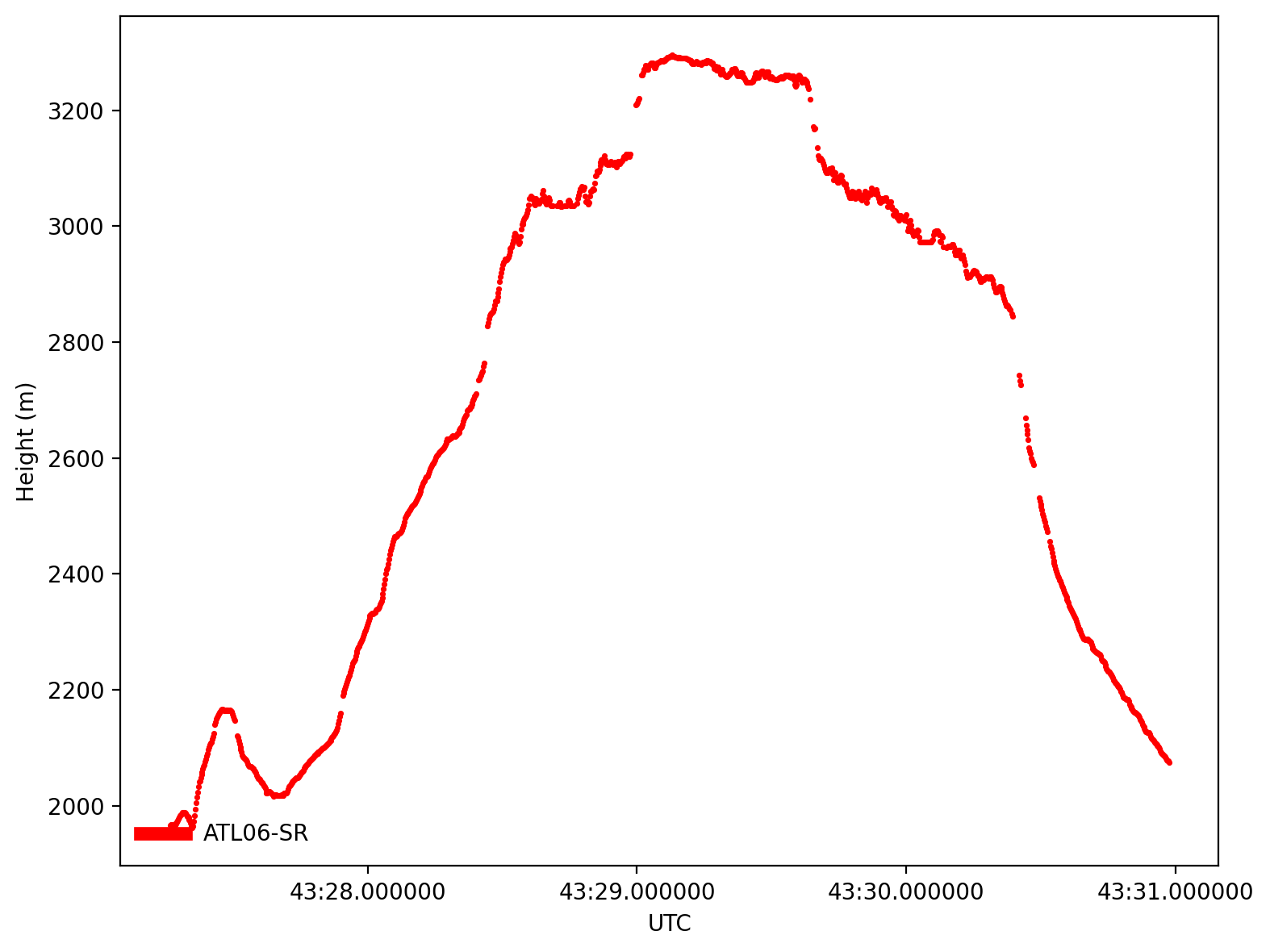

Advanced ICESat-2 SlideRule Example: Polar Altimetry and Raster Sampling¶

SlideRule also can use different sources for photon classification before calculating the average segment height.
This is useful for example, in cases where there may be a vegetated canopy affecting the spread of the photon returns.

ATL03 photon confidence values, based on algorithm-specific classification types for land, ocean, sea-ice, land-ice, or inland water
ATL08 Land and Vegetation Height product photon classification
Experimental YAPC (Yet Another Photon Classification) photon-density-based classification

For this example, we will also use SlideRule to sample a digital elevation model (DEM) at the locations of our ICESat-2 elevations. For a detailed discussion of the raster sampling capability see the GeoRaster page and the sampling parameters in the SlideRule documentation.

SlideRule does not currently include first-photon bias or transmit-pulse shape bias corrections in the fit heights.

Leaflet Basemaps and Layers¶

There are 3 projections available within SlideRule for mapping (Global, North and South). There are also contextual layers available for each projection. Most xyzservice providers can be added as contextual layers to the global Web Mercator maps.

Global (Web Mercator, EPSG:3857)	North (Alaska Polar Stereographic, EPSG:5936)	South (Antarctic Polar Stereographic, EPSG:3031)
USGS 3DEP Hillshade ASTER GDEM Hillshade ESRI Imagery Global Land Ice Measurements from Space (GLIMS) Randolph Glacier Inventory (RGI)	ESRI Imagery ArcticDEM	Landsat Image Mosaic of Antarctica (LIMA) MODIS Mosaic of Antarctica (MOA) Radarsat Antarctic Mapping Project (RAMP) Reference Elevation Model of Antarctica (REMA)

Here, we will use the visualize data at Fenris Glacier in Greenland using the Northern Hemisphere polar stereographic projection.

# create ipyleaflet map in specified projection
m2 = sliderule.ipysliderule.leaflet('North',
    center=(66.55, -36.75), zoom=8)
# add ArcticDEM Hillshade layer
m2.add_layer(
    layers='ArcticDEM',
    rendering_rule={'rasterFunction': 'Hillshade Gray'}
)
# read and add region of interest
reg = gpd.read_file('Fenris_Gletscher_PS_v1.4.2.geojson')
m2.add_region(sliderule.io.from_geodataframe(reg))
m2.map

Update options for making science data processing requests to SlideRule¶

Here we’ll be able to adjust all the potential parameters for making a SlideRule ICESat-2 atl06 request.

Parameter	Definition
Classification	Photon classification types to use in signal selection atl03: signal confidence quality: signal quality flag atl08: classification from the land and vegetation algorithm yapc: confidence determined using a clustering algorithm
Surface Type	Sets the parameters for ATL03 photon confidence classification land ocean sea ice land ice inland water
Confidence	Numerical assessment of the signal likelihood of each photon photon is background photon is background within buffer of known surface low confidence of photon being signal medium confidence of photon being signal high confidence of photon being signal
Quality	ATL03 instrumental photon quality photon is nominal photon is possible afterpulse photon is possible impulse response photon is possible transmit echo path (TEP)
Land class	ATL08 land and vegetation classification photon is noise or background photon is ground photon is canopy photon is top of canopy photon is not classified
YAPC kNN	Number of nearest neighbors to use in classification algorithm Automatic selection
YAPC h window	Window height for filtering neighbors in classification algorithm
YAPC x window	Window width for filtering neighbors in classification algorithm
YAPC minimum PE	Minimum number of photon events needed to create a YAPC score in classification algorithm
YAPC score	Minimum YAPC score for photons to be valid
Length	How long each segment should be in meters
Step	Distance between successive segments in meters
PE Count	Minimum number of photon events needed within a segment to be valid
Window	Minimum height of the final surface window used for selecting photons
Sigma	Maximum allowed dispersion around the median height in meters

# display widgets for setting SlideRule parameters
SRwidgets.set_atl06_defaults()
SRwidgets.classification.value = ['atl03']
SRwidgets.surface_type.value = 'Land ice'
SRwidgets.VBox(SRwidgets.atl06())

%%time
# build sliderule parameters using latest values from widget
parms = SRwidgets.build_atl06()
# reduce data to a single cycle
parms["cycle"] = 19
# additionally sample ArcticDEM mosaic at ATL06-SR points
parms["samples"] = dict(mosaic= {
    "asset": "arcticdem-mosaic",
    "radius": 10.0,
    "zonal_stats": True
})

# clear existing geodataframe results
elevations = [sliderule.emptyframe()]

# for each region of interest
for poly in m2.regions:
    # add polygon from map to sliderule parameters
    parms["poly"] = poly
    # make the request to the SlideRule (ATL06-SR) endpoint
    # and pass it the request parameters to request ATL06 Data
    elevations.append(sliderule.icesat2.atl06p(parms))
# concatenate the results into a single geodataframe
gdf2 = gpd.pd.concat(elevations)

HTTP Request Error: Request Entity Too Large
Using simplified polygon (for CMR request only!), 457 points using tolerance of 0.0001
HTTP Request Error: Request Entity Too Large
Using simplified polygon (for CMR request only!), 375 points using tolerance of 0.001
HTTP Request Error: Request Entity Too Large
Using simplified polygon (for CMR request only!), 73 points using tolerance of 0.01

CPU times: user 3.49 s, sys: 109 ms, total: 3.6 s
Wall time: 1min 21s

Add GeoDataFrame to polar stereographic map¶

# ATL06-SR fields for hover tooltip
fields = m2.default_atl06_fields()
gdf2.leaflet.GeoData(m2.map, column_name=SRwidgets.column_name, cmap=SRwidgets.colormap,
    max_plot_points=10000, tooltip=True, colorbar=True, fields=fields)
# install handlers and callbacks
gdf2.leaflet.add_selected_callback(SRwidgets.atl06_click_handler)
m2.add_region_callback(gdf2.leaflet.handle_region)

Create a static map with SlideRule returns¶

Here, we’re going to create a static map of Fenris Glacier in Greenland with our SlideRule returns from ICESat-2 and ArcticDEM. We’re going to plot the data in a different Polar Stereographic projection (NSIDC Sea Ice Polar Stereographic North). geopandas GeoDataFrames can be transformed to different Coordinate Reference Systems (CRS) using the to_crs() function.

def plot_arcticdem(ax=None, **kwargs):
    """Plot ArcticDEM layer as a basemap

    Parameters
    ----------
    ax: obj, default None
        Figure axis
    kwargs: dict, default {}
        Additional keyword arguments for ``wms.getmap``
    """
    # set default keyword arguments
    kwargs.setdefault('layers', '0')
    kwargs.setdefault('format', 'image/png')
    kwargs.setdefault('srs', 'EPSG:3413')
    # create figure axis if non-existent
    if (ax is None):
        _, ax = plt.subplots()
    # get the pixel bounds and resolution of the map
    width = int(ax.get_window_extent().width)
    height = int(ax.get_window_extent().height)
    # calculate the size of the map in pixels
    kwargs.setdefault('size', [width, height])
    # calculate the bounding box of the map in projected coordinates
    bbox = [None]*4
    bbox[0], bbox[2] = ax.get_xbound()
    bbox[1], bbox[3] = ax.get_ybound()
    kwargs.setdefault('bbox', bbox)
    # url of ArcticDEM WMS
    url = ('http://elevation2.arcgis.com/arcgis/services/Polar/'
        'ArcticDEM/ImageServer/WMSserver')
    wms = owslib.wms.WebMapService(url=url, version='1.1.1')
    basemap = wms.getmap(**kwargs)
    # read WMS layer and plot
    img = plt.imread(io.BytesIO(basemap.read()))
    ax.imshow(img, extent=[bbox[0],bbox[2],bbox[1],bbox[3]])

# create polar stereographic plot of ATL06-SR data
# EPSG codes are a simple way to define many coordinate reference systems
crs = 'EPSG:3413'
# create figure axis
fig,ax1 = plt.subplots(num=1, ncols=3, sharex=True, sharey=True, figsize=(13,3.5))
ax1[0].set_aspect('equal', adjustable='box')

# calculate normalization for height plots
vmin, vmax = gdf2['h_mean'].quantile((0.02, 0.98)).values

# calculate difference between sliderule and ArcticDEM mosaic heights
gdf2['difference'] = gdf2['h_mean'] - gdf2['mosaic.mean']
filtered = gdf2[gdf2['difference'].abs() < 100].to_crs(crs)

# plot ATL06-SR elevation
ax1[0].set_title('ATL06-SR')
label = f'Elevation [m]'
sc = filtered.plot(ax=ax1[0], zorder=1, markersize=0.5,
    column='h_mean', cmap='plasma_r', vmin=vmin, vmax=vmax,
    legend=True, legend_kwds=dict(label=label, shrink=0.90, extend='both'))
sc.set_rasterized(True)

# plot ArcticDEM mosaic elevation
ax1[1].set_title('ArcticDEM Mosaic')
label = f'Elevation [m]'
sc = filtered.plot(ax=ax1[1], zorder=1, markersize=0.5,
    column='mosaic.mean', cmap='plasma_r', vmin=vmin, vmax=vmax,
    legend=True, legend_kwds=dict(label=label, shrink=0.90, extend='both'))
sc.set_rasterized(True)

# plot difference between heights
ax1[2].set_title('ATL06-SR - ArcticDEM')
label = f'Elevation Difference [m]'
sc = filtered.plot(ax=ax1[2], zorder=1, markersize=0.5,
    column='difference', cmap='coolwarm', vmin=-30, vmax=30,
    legend=True, legend_kwds=dict(label=label, shrink=0.90, extend='both'))
sc.set_rasterized(True)

# convert regions into a geoseries object
regions = []
for poly in m2.regions:
    lon,lat = sliderule.io.from_region(poly)
    regions.append(shapely.geometry.Polygon(zip(lon,lat)))
gs = gpd.GeoSeries(regions, crs='EPSG:4326').to_crs(crs)

# add background and labels
for ax in ax1:
    # plot each region of interest
    gs.plot(ax=ax, facecolor='none', edgecolor='black', lw=3)
    # plot ArcticDEM as basemap
    plot_arcticdem(ax, srs=crs)
    # add x label
    ax.set_xlabel('{0} [{1}]'.format('Easting','m'))
# add y label
ax1[0].set_ylabel('{0} [{1}]'.format('Northing','m'))

# adjust subplot and show
fig.subplots_adjust(left=0.06, right=0.98, bottom=0.08, top=0.98, wspace=0.1)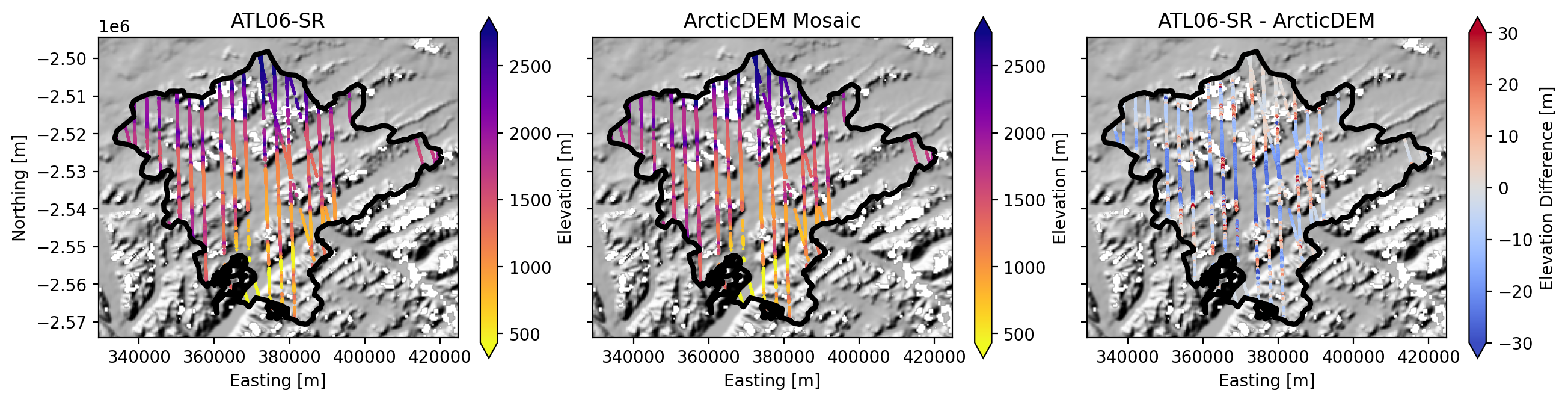

Advanced ICESat-2 SlideRule Example: PhoREAL Vegetation Metrics¶

For this example, we will also use SlideRule to produce canopy metrics using the ATL08 PhoREAL API. The name comes from the University of Texas team that developed PhoREAL and collaborated with us to get their algorithms into SlideRule. The PhoREAL functionality within SlideRule uses the land surface classifications for each photon provided by the ICESat-2 Land and Vegetation Height Product (ATL08). Similar to the SlideRule elevation functionality, these metrics can be calculated at different lengths scales and with different options for classification. The set of parameters specific to the ATL08 processing are provided under the phoreal key.

Documentation for this functionality can be found in the API reference.

# create ipyleaflet map in specified projection
m3 = sliderule.ipysliderule.leaflet('Global', zoom=10,
    full_screen_control=True)
# add ESRI imagery layer
m3.add_layer(layers=['ESRI imagery'])
# read and add region of interest
reg = gpd.read_file('grandmesa.geojson')
m3.add_region(sliderule.io.from_geodataframe(reg))
m3.map

Set options for making PhoREAL science data processing requests to SlideRule¶

Here, we’ll be able to adjust all the potential parameters for making a SlideRule ICESat-2 atl08 request.

Parameter	Definition
Classification	Photon classification types to use in signal selection atl03: signal confidence quality: signal quality flag atl08: classification from the land and vegetation algorithm yapc: confidence determined using a clustering algorithm
Land class	ATL08 land and vegetation classification photon is noise or background photon is ground photon is canopy photon is top of canopy photon is not classified
PhoREAL Bin Size	Size of the vertical histogram bin in meters
PhoREAL Geolocation	Method for calculating segment geolocation variables mean: average value across all photons in the segment median: median value across all photons in the segment center: center of first and last photons in the segment
PhoREAL Use abs h	Use absolute photon event elevations rather than normalized heights
PhoREAL ABoVE	Use the ABoVE photon classifier
PhoREAL Waveform	Return the photon height histograms
Length	How long each segment should be in meters
Step	Distance between successive segments in meters

# display widgets for setting SlideRule parameters
SRwidgets.set_atl08_defaults()
SRwidgets.VBox(SRwidgets.atl08())

%%time
# build sliderule parameters using latest values from widget
parms = SRwidgets.build_atl08()
# reduce data to a single cycle
parms["cycle"] = 16

# clear existing geodataframe results
elevations = [sliderule.emptyframe()]

# for each region of interest
for poly in m3.regions:
    # add polygon from map to sliderule parameters
    parms["poly"] = poly
    # make the request to the SlideRule (ATL08-SR) endpoint
    # and pass it the request parameters to request ATL08 vegetation metrics
    elevations.append(sliderule.icesat2.atl08p(parms, keep_id=True))
# concatenate the results into a single geodataframe
gdf3 = gpd.pd.concat(elevations)

CPU times: user 1.06 s, sys: 23.5 ms, total: 1.09 s
Wall time: 12.7 s

Review GeoDataFrame output¶

There are different columns for the atl08 request, which add the vegetation metrics. Here, we will inspect the top of the ATL08 GeoDataFrame using head().

See the SlideRule ICESat-2 Vegetation Metrics documentation for descriptions of each column

print(f'Returned {gdf3.shape[0]} records')
gdf3.head()

Add Vegetation Metrics GeoDataFrame to map¶

Here, we’re going to visualize the canopy height h_canopy. This is the 98^th percentile of the histogram of canopy photons that are located above the Earth’s surface.

SRwidgets.VBox([
    SRwidgets.variable,
    SRwidgets.cmap,
    SRwidgets.reverse,
])

# ATL06-SR fields for hover tooltip
fields = m3.default_atl08_fields()
gdf3.leaflet.GeoData(m3.map, column_name=SRwidgets.column_name, cmap=SRwidgets.colormap,
    max_plot_points=10000, tooltip=True, tooltip_width='280px', colorbar=True,
    fields=fields)
# install handlers and callbacks
gdf3.leaflet.add_selected_callback(SRwidgets.atl06_click_handler)
m3.add_region_callback(gdf3.leaflet.handle_region)

Advanced ICESat-2 SlideRule Example: Subsetting ATL03 photon cloud data¶

SlideRule can also be used to subset ATL03 geolocated photon height products, which are returned as a geopandas GeoDataFrame at the photon rate. Documentation for this function can be found in the API reference.

Because each granule contains so many photons, it is good practice to subset the data as much as possible by limiting the subsetting area and the number of granules to be processed. Here, we supply a GeoJSON file of Fenris Glacier for trimming the photon data. We also supply a reference ground track and cycle number to reduce the number of granules to be processed to a single file. Finally, we specify that only tracks GT1L and GT1R within the granule should be subset. This will still return hundreds of thousands of photons for the region!

The other parameters in the request are used to specify different aspects of the ATL03 subsetting request. The surface type for photon classification (srt) in this case is land ice. This surface type parameter is used in conjunction the photon confidence level cnf parameter. Here, we are requesting that all classified photons for the surface type are returned.

# read Region of Interest
reg = gpd.read_file('Fenris_Gletscher_PS_v1.4.2.geojson')
region = sliderule.io.from_geodataframe(reg)
RGT = 71
cycle = 19
# only process data for GT1L and GT1R
PT = 1

# Build ATL03 Subsetting Request Parameters
parms = {
    "poly": region[0],
    "rgt": RGT,
    "cycle": cycle,
    "track": PT,
    "srt": sliderule.icesat2.SRT_LAND_ICE,
    "cnf": sliderule.icesat2.CNF_BACKGROUND,
    "len": 20.0,
    "pass_invalid": True
}

# Make ATL03 Subsetting Request
atl03 = sliderule.icesat2.atl03sp(parms)

HTTP Request Error: Request Entity Too Large
Using simplified polygon (for CMR request only!), 457 points using tolerance of 0.0001
HTTP Request Error: Request Entity Too Large
Using simplified polygon (for CMR request only!), 375 points using tolerance of 0.001
HTTP Request Error: Request Entity Too Large
Using simplified polygon (for CMR request only!), 73 points using tolerance of 0.01

Review GeoDataFrame output¶

The ATL03 GeoDataFrame will have variables at the photon rate. Here, we will inspect the columns and variables at the top of the ATL03 GeoDataFrame using head(). See the SlideRule ICESat-2 Geolocated Photon documentation for descriptions of each column

print(f'Returned {atl03.shape[0]} records')
atl03.head()

Create plot for a single track of photon heights¶

Here, we’re going to use the same SlideRule ICESat-2 transect plot functionality as prior, but for visualizing the geolocated photons.

scatter: Will plot ATL03 data returned by SlideRule for a single RGT, ground track and cycle

atl03.icesat2.plot(atl03='dataframe', kind='scatter', title='ATL03 Photon Cloud',
    legend=True, legend_frameon=True,
    classification='atl03', segments=False,
    RGT=RGT, cycle=cycle, GT=sliderule.icesat2.GT1R)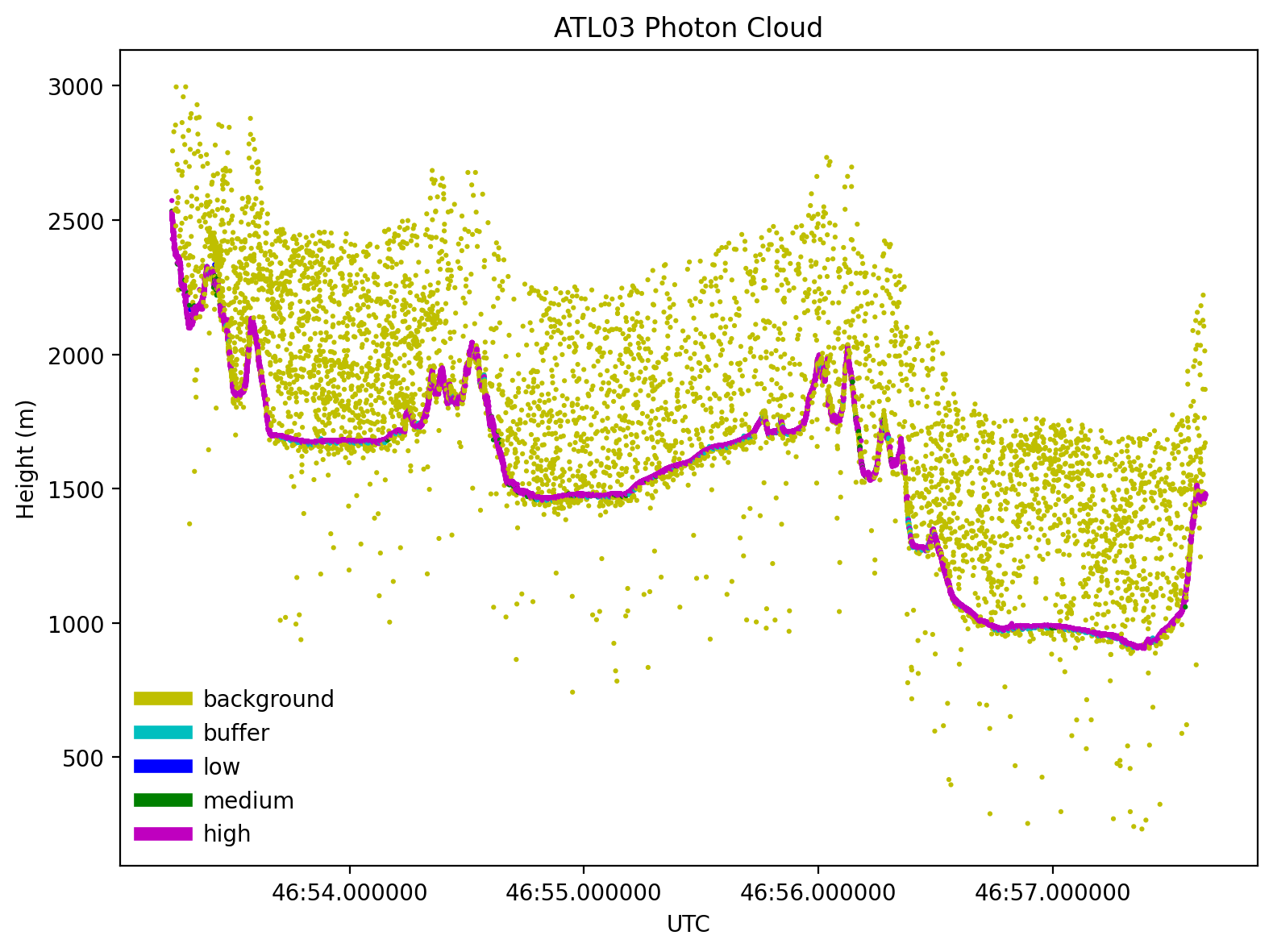

Direct File Read Example¶

SlideRule also can directly read data from HDF5 files stored in s3 using h5coro, a cloud-optimized HDF5 reader built by the SlideRule team. In the example below, data from the first 25 segments are read from an ATL06 granule. The results are returned in a dictionary of arrays, where each key is the name of the dataset. The entirety of a dataset can be read by setting the number of rows to h5.ALL_ROWS.

resource = 'ATL06_20181017222812_02950102_006_02.h5'
beams = ['gt1l', 'gt1r', 'gt2l', 'gt2r', 'gt3l', 'gt3r']
variables = ['latitude', 'longitude']
startrow, numrows = (0, 25)
datasets = [dict(dataset=f'/{b}/land_ice_segments/{v}', startrow=startrow, numrows=numrows)
    for b in beams for v in variables]
atl06 = sliderule.h5.h5p(datasets, resource, 'icesat2')

fig, ax2 = plt.subplots(num=2, figsize=(6,6))
for b in beams:
    ax2.plot(atl06[f'/{b}/land_ice_segments/longitude'],
        atl06[f'/{b}/land_ice_segments/latitude'],
        '.-', ms=5, lw=0, label=b)
ax2.set_title(resource)
ax2.set_xlabel('Longitude [\u00B0]')
ax2.set_ylabel('Latitude [\u00B0]')
lgd = ax2.legend(frameon=False)
lgd.get_frame().set_alpha(1.0)
for line in lgd.get_lines():
    line.set_linewidth(6)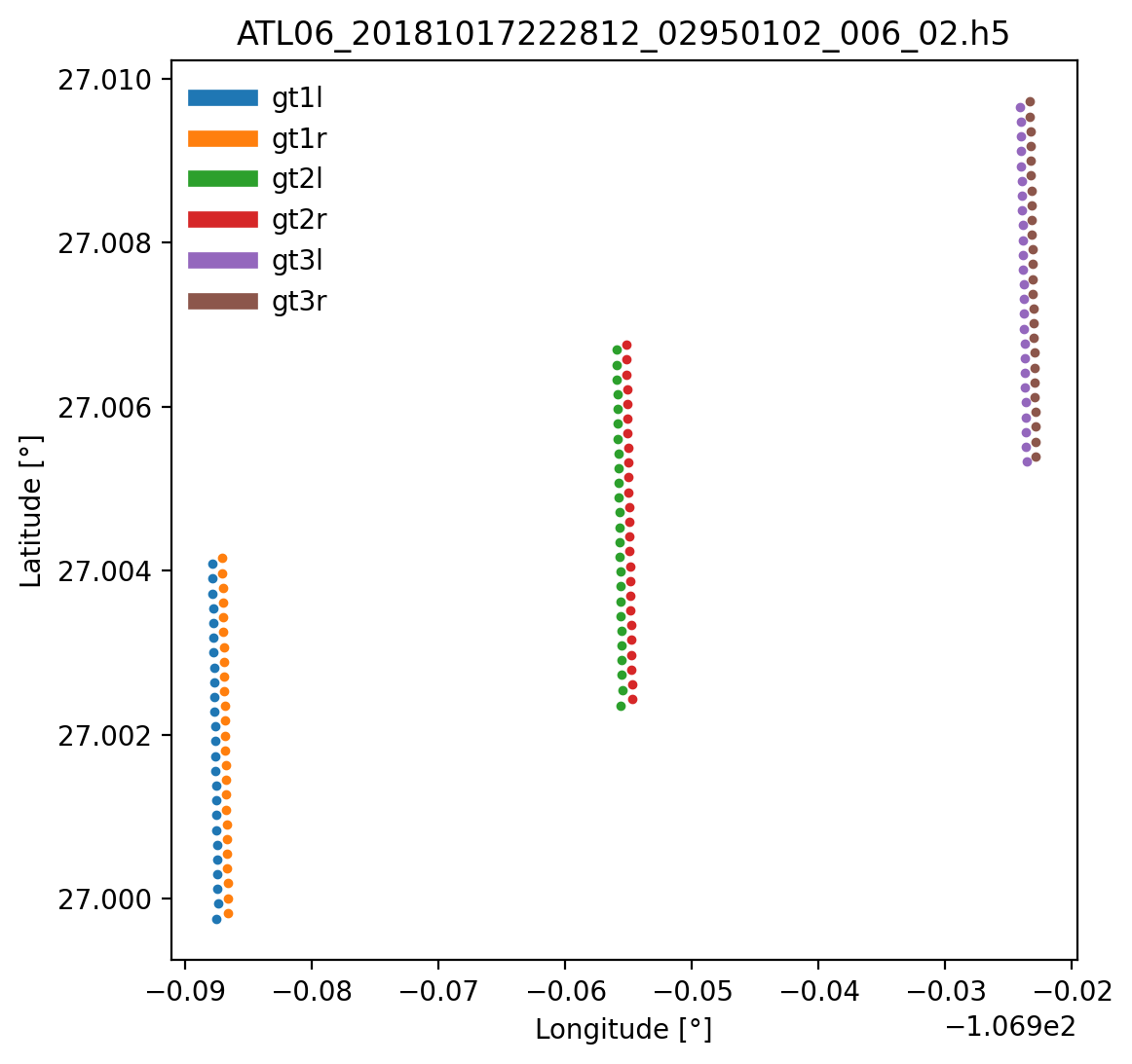

Private Clusters¶

The SlideRule project supports the deployment of private clusters. A private cluster is a separate deployment of the public SlideRule service with the only difference being it requires authenticated access. These clusters are managed through the SlideRule Provisioning System and require both an account on that system along with an association with a funding organization. For more information on private clusters, please see the users guide.

The public SlideRule service is provisioned the exact same way as a private cluster and is managed by the SlideRule Provisioning System. Each cluster has its own subdomain and configuration. For the public cluster, the configuration specifies that no authentication is needed, and the subdomain is “sliderule”, so access to the public cluster is at https://sliderule.slideruleearth.io. For the other clusters, access requires authentication and the subdomain is the set to the name of the organization funding the cluster. For example, the University of Washington private cluster is at https://uw.slideruleearth.io.

Summary¶

SlideRule is a cost-effective science data as a service solution that provides responsive results to users. SlideRule can enable large scale access to the NASA and other Earth science data and provide science-quality algorithms in an open and documented way. The SlideRule team strives to provide simple, well-documented APIs that are easy to install and use, as well as a web client for online demonstration. Improvements and fixes can be made quickly to limit downtime and enable new functionality. The SlideRule system is highly scalable to meet the processing demand at any given time. In addition, private clusters can be made available to users for large-scale requests. See more at slideruleearth.io.

Details

Part 2b: Using the icepyx python library to access ICESat-2 data (ATL06)

Details

Parallelized Cloud Computing with Dask for Geoscientists