Loading Raster Data from GeoTIFF Files

Given that most of the geospatial data we’ll work with in this tutorial is stored in GeoTIFF files, we need to know how to work with those files. The easiest solution is to use rioxarray; this solution takes care of a lot of tricky details transparently. We can also use Rasterio as a tool for reading data or metadata from GeoTIFF files; judicious use of Rasterio can make a big difference when working with remote files in the cloud.

rioxarray¶

rioxarray is a package that extends the Xarray package (more on that later). The primary rioxarray features we’ll use within this tutorial are:

• rioxarray.open_rasterio to load GeoTIFF files directly into Xarray DataArray structures; and
• xarray.DataArray.rio to provides useful utilities (e.g., for specifying CRS information).

To get used to working with GeoTIFF files, we’ll use a few specific examples in this & later notebooks. We’ll explain more about what kind of data is contained within the file later; for now, we just want to get used to loading data.

Loading files into a DataArray¶

Observe first that open_rasterio works on local file paths and remote URLs.

• Predictably, local access is faster than remote access.

This next operation compares elements of an Xarray DataArray elementwise (the use of the .all method is similar to what we would do to compare NumPy arrays). This is generally not an advisable way to compare arrays, series, dataframes, or other large data structures that contain floating-point data. However, in this particular instance, as the two data structures have been read from the same file stored in two different locations, element-by-element comparison makes sense. It confirms that the data loaded into memory from two different sources is identical in every bit.

rasterio¶

This section can be safely skipped if rioxarray works adequately for our analyses, i.e., if loading data into memory is not prohibitive; when that is not the case, rasterio provides alternative strategies for exploring GeoTIFF files. That is, the rasterio package offers lower-level approaches to loading data than rioxarray does when needed.

From the Rasterio documentation:

Before Rasterio there was one Python option for accessing the many different kind of raster data files used in the GIS field: the Python bindings distributed with the Geospatial Data Abstraction Library, GDAL. These bindings extend Python, but provide little abstraction for GDAL’s C API. This means that Python programs using them tend to read and run like C programs. For example, GDAL’s Python bindings require users to watch out for dangling C pointers, potential crashers of programs. This is bad: among other considerations we’ve chosen Python instead of C to avoid problems with pointers.

What would it be like to have a geospatial data abstraction in the Python standard library? One that used modern Python language features and idioms? One that freed users from concern about dangling pointers and other C programming pitfalls? Rasterio’s goal is to be this kind of raster data library – expressing GDAL’s data model using fewer non-idiomatic extension classes and more idiomatic Python types and protocols, while performing as fast as GDAL’s Python bindings.

High performance, lower cognitive load, cleaner and more transparent code. This is what Rasterio is about.

Opening files with rasterio.open¶

Given a data source (e.g., a GeoTIFF file in the current context), we can open a DatasetReader object associated with using rasterio.open. Technically, we have to remember to close the object afterward. That is, our code would look like this:

As with file-handling in Python, we can use a context manager (i.e., a with clause) instead.

with rasterio.open(LOCAL_PATH) as ds:
  # ...
  # do some computation
  # ...

# more code outside the scope of the with block.

The dataset will be closed automatically outside the with block.

The principal advantage of using rasterio.open rather than rioxarray.open_rasterio to open a file is that the latter approach opens the file and immediately loads its contents into a DataDarray in memory.

By contrast, using rasterio.open opens the file in place and its contents are not immediately loaded into memory. The file’s data can be read, but this must be done explicitly. This makes a lot of difference when working with remote data; transferring the entire contents across a network involves certain costs. For example, if we examine the metadata—which is typically much smaller and can be transferred quickly—we may find, e.g., that moving an entire array of data across the network is not warranted.

Examining DatasetReader attributes¶

When a file is opened using rasterio.open, the object instantiated is from the DatasetReader class. This class has a number of attributes and methods of interest to us:

First, given a DatasetReader ds associated with a data source, examining ds.profile returns some diagnostic information.

The attributes ds.height, ds.width, ds.shape, ds.count, ds.nodata, and ds.transform are all included in the output from ds.profile but are also accessible individually.

Reading data into memory¶

The method ds.read loads an array from the data file into memory. Notice this can be done on local or remote files.

The array loaded into memory with ds.read is a NumPy array. This can be wrapped by an Xarray DataArray if we provide additional code to specify the coordinate labels and so on.

Mapping coordinates¶

Earlier, we loaded data from a local file into a DataArray called da using rioxarray.open_rasterio.

Doing so simplified the loading raster data from a GeoTIFF file into an Xarray DataArray while filling in the metadata for us. In particular, the coordinates associated with the pixels were stored into da.coords (the default coordinate axes are band, x, and y for this three-dimensional array).

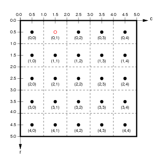
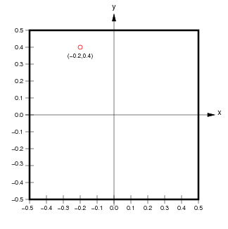
If we ignore the extra band dimension, the pixels of the raster data are associated with pixel coordinates (integers) and spatial coordinates (real values, typically a point at the centre of each pixel).

(from http://ioam.github.io/topographica)

The accessors da.isel and da.sel allow us to extract slices from the data array using pixel coordinates or spatial coordinates respectively.

If we use rasterio.open to open a file, the DatasetReader attribute transform provides the details of how to convert between pixel and spatial coordinates. We will use this capability in some of the case studies later.

The attribute ds.transform is an object describing an affine transformation (represented above as a $2\times3$ matrix). Notice that the absolute values of the diagonal entries of the matrix ds.transform give the spatial dimensions of pixels ($30\mathrm{m}\times30\mathrm{m}$ in this case).

We can also use this object to convert pixel coordinates to the corresponding spatial coordinates.

The attribute ds.bounds displays the bounds of the spatial region (left, bottom, right, top).

The method ds.xy also converts integer index coordinates to continuous coordinates. Notice that ds.xy maps integers to the centre of pixels. The loops below print out the first top left corner of the coordinates in pixel coordinates and then the cooresponding spatial coordinates.

ds.index does the reverse: given spatial coordinates (x,y), it returns the integer indices of the pixel that contains that point.

These conversions can be tricky, particularly because pixel coordinates map to the centres of the pixels and also because the second y spatial coordinate decreases as the second pixel coordinate increases. Keeping track of tedious details like this is partly why loading from rioxarray is useful, i.e., this is done for us. But it is worth knowing that we can reconstruct this mapping if needed from metadata in the GeoTIFF file (we use this fact later).