Working with Vector Data

Certain physical properties of interest in GIS are not conveniently captured by raster data on discrete grids. For instance, geometric features of a landscape like roads, rivers and boundaries between regions are better described using lines or curves in a suitable projected coordinate system. Vector data, in the context of GIS, refers to geometric representations of such aspects of a landscape.

Understanding Vector Data¶

Vector data consists of ordered sequences of vertices, i.e., pairs of numbers of the form $(x,y)$. The continuous coordinates of each vertex are associated with a physical spatial location in some projected CRS (Coordinate Reference System).

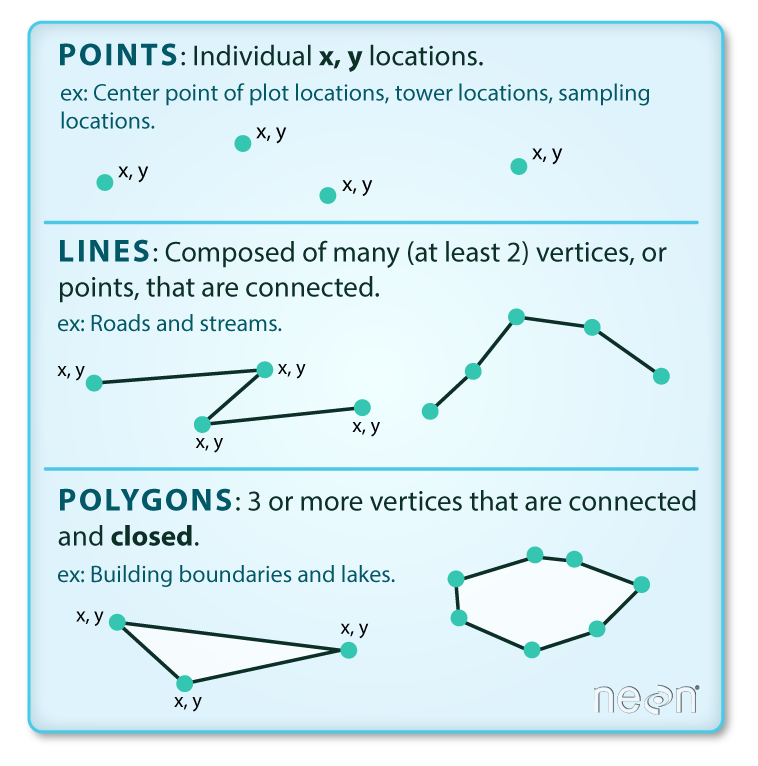
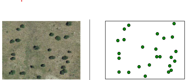
• Point data: Isolated vertices represent discrete zero-dimensional features (e.g., trees, street lamps, etc.).
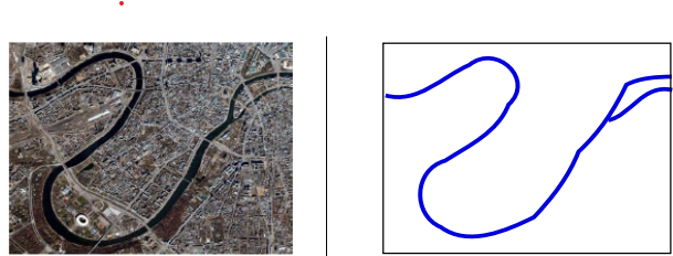
• Line data: Any ordered sequence of at least two vertices constitutes a “polyline” that can be visualized by drawing straight lines between adjacent vertices. Line data is suitable for representing one-dimensional features like roads, trails, and rivers.
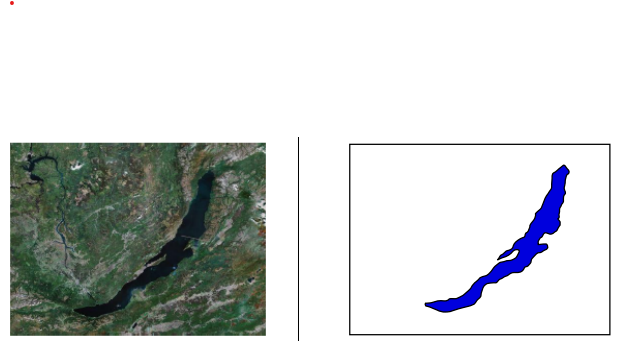
• Polygon data: Any ordered sequence of at least three vertices in which the first and last vertex are the same constitutes a polygon (i.e., a closed shape). Polygon data is suitable for describing two-dimensional regions like a lake or the boundary of a forest. A common use of polygon data is to represent borders between political constituencies (e.g., countries).

A single vector dataset georeferenced with a particular CRS typically contains any number of points, lines, or polygons.

This image shows the three vector types: points, lines and polygons. Source: National Ecological Observatory Network.

(Left image) Overhead view of a landscape; (right image) Point vector representations of salient features.
Source: *Sistemas de Información Geográfica* by Victor Olaya.

(Left image) Overhead view of a river; (right image) Line vector representation of the river.
Source: *Sistemas de Información Geográfica* by Victor Olaya.

(Left image) Overhead view of a lake; (right image) Polygon vector representation of the lake
Source: *Sistemas de Información Geográfica* by Victor Olaya.

As with raster data, vector data representations are usually bundled with metadata to store various attributes associated with the dataset. Vector data is generally specified at a higher level of precision than the resolution than most raster grids allow. Moreover, geographic features represented as vector data enables computations that raster data does not. For instance, it is possible to determine various geometric or topological relationships:

• Does a point lie within the boundary of a geographic region?
• Do two roads intersect?
• What is the nearest point on a road to another region?

Other geometric quantities like the length of a river or the surface area of a lake are available by applying techniques from computational geometry to vector data representations.

Using GeoJSON¶

GeoJSON is a subset of JSON (JavaScript object notation). It was developed in the early 2000s to represent simple geographical features together with non-spatial attributes. The core idea is to provide a specification for encoding geospatial data that can be decoded by any JSON decoder.

The GIS developers responsible for GeoJSON designed it with the intention that any web developer should be able to write a custom GeoJSON parser, allowing for many possible ways to use geospatial data beyond standard GIS software. The technical details of the GeoJSON format are described in the standards document RFC7946.

Let’s see how to parse and plot GeoJSON files using GeoPandas. The local file cables.geojson stores line vector data representing underwater cables connecting different land masses.

Trying to read the GeoJSON output above is tricky but predictable. JSON files are generically intended for machine consumption and are hence not very readable.

Let’s use the geopandas.read_file function to load the vector data into a GeoDataFrame.

There are 530 rows each of which corresponds to line data (a connected sequence of line segments). We can use the GeoDataFrame column color as an option within a call to .plot to make a plot of these cables.

Let’s use a remote file to create another GeoDataFrame, this time containing polygon data.

This time, the plot shows filled polygons corresponding to the countries of the world.

The GeoDataFrame.loc accessor allows us to plot particular subsets of countries.

Using Shapefiles¶

The shapefile standard is a digital format for distributing geospatial vector data and its associated attributes. The standard—first developed by ESRI roughly 30 years ago—is supported by most modern GIS software tools. The name “shapefile” is a bit misleading because a “shapefile” typically consists of a bundle of several files (some mandatory, some optional) stored in a common directory with a common filename prefix.

From Wikipedia:

The shapefile format stores the geometry as primitive geometric shapes like points, lines, and polygons. These shapes, together with data attributes that are linked to each shape, create the representation of the geographic data. The term “shapefile” is quite common, but the format consists of a collection of files with a common filename prefix, stored in the same directory. The three mandatory files have filename extensions .shp, .shx, and .dbf. The actual shapefile relates specifically to the .shp file, but alone is incomplete for distribution as the other supporting files are required. Legacy GIS software may expect that the filename prefix be limited to eight characters to conform to the DOS 8.3 filename convention, though modern software applications accept files with longer names.

Shapefiles use the Well-Known Binary (WKB) format for encoding geometries. This is a compact tabular format, i.e., row and column numbers ass value is significant. Some minor limitations of this format include the restriction of attribute field names to 10 characters or fewer and poor Unicode support; as a result, text is often abbreviated and encoded in ASCII.

You can refer to the ESRI Shapefile Technical Whitepaper to find out more about shapefiles.

Mandatory files¶

• Main File (.shp): shape format, i.e., the spatial vector data (points, lines, and polygons) representing feature geometry.
• Index File (.shx): shape index positions (to enable retrieval of feature geometry).
• dBASE File (.dbf): standard database file storing attribute format (columnar attributes for each shape in dBase IV format, typically readable by, e.g., Microsoft Access or Excel).

Records correspond in sequence in each of these files , i.e., attributes in record $k$ of the dbf file describe the feature in record $k$ of the associated shp file.

Optional files¶

• Projection File (.prj): description of relevant coordinate reference system using a well-known text (WKT or WKT-CRS) representation.
• Extensible Markup Language File (.xml): geospatial metadata in XML format.
• Code Page File (.cpg): plain text files to describe the encoding applied to create the shapefile. If your shapefile doesn’t have a .cpg file, then it has the system´s default encoding.
• Spatial Index Files (.sbn and .sbx): encoded index files to speed up loading times.

There are numerous other optional files; see the whitepaper.

As with GeoJSON files, shapefiles can be read directly using geopandas.read_file to load the .shp file. We’ll do this now using an example shapefile that shows the boundary of a wildfire.

We’ll use this particular shapefile again in later notebooks and explain what it represents in greater detail then.