Working with Raster Data

From the Wikipedia description of raster graphics:

In computer graphics and digital photography, a raster graphic represents a two-dimensional picture as a rectangular matrix or grid of pixels, viewable via a computer display, paper, or other display medium.

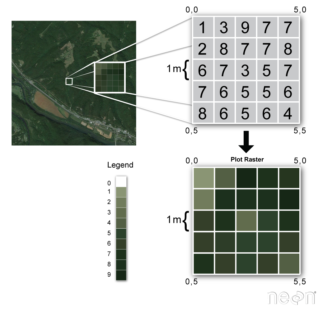
The term “raster data” or “raster” originated in computer graphics; in essence, a raster refers to a sequence of numerical values arranged into a rectangular table (similar to a matrix from linear algebra).

Raster datasets are useful to represent continuous quantities—pressure, elevation, temperature, land cover classification, etc.—sampled on a tesselation, i.e, a discrete grid that partitions a two-dimensional region of finite extent. In the context of Geographic Information Systems (GIS), the spatial region is planar projection of a portion of the Earth’s surface.

Rasters approximate continuous numerical distributions by storing individual values within each grid cell or pixel (a term derived from “picture element” in computer graphics). Rasters can represent data gathered over various types of non-rectangular grid cells (e.g., hexagons); for our purposes, we’ll restrict our attention to grids in which all the pixels are rectangles of the same height and width.

This image shows an example of raster data. Source: National Ecological Observatory Network (NEON).

Understanding Raster Values¶

An important subtle difference between a numerical matrix familiar from linear algebra and a raster in the context of GIS is that real datasets are often incomplete. That is, a raster may have entries missing or it may include pixel values that were corrupted during the measurement process. As such, most raster data includes a scheme to represent “No Data” values for any pixels where no meaningful observation is possible. The scheme may use ‘NaN’ (“Not-a-Number”) for floating-point data or a sentinel value for integer data (e.g., using -1 to signal missing data where meaningful integer data is strictly positive).

Another important property of raster data is that pixel values are stored using an appropriate data type for the context. For instance, continuous features like elevation or temperature would often be stored as raster data using floating-point numbers; by contrast, categorical properties (like land cover types) may be stored using unsigned integers. Raster datasets are often large, so choosing the data type judiciously can reduce file size significantly without compromising the quality of information. We shall see this in examples later.

Understanding Pixel vs. Continuous Coordinates¶

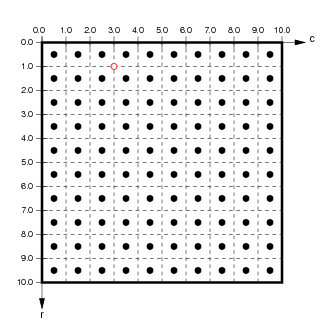
Each pixel of a raster data set is indexed by its row & column position relative to the top left corner — the image or pixel coordinates. These values represent the displacement from the top left corner of the matrix, conventionally expressed using zero-based numbering. For instance, using zero-based indexing in the $10\times10$ grid of pixels displayed below, the top left corner pixel has index (0,0); the top right corner pixel has index (0,9); the bottom left corner pixel has index (9,0); and the bottom right corner pixel has index (9,9).

(from http://ioam.github.io/topographica)

Zero-based indexing is not observed universally (e.g., MATLAB uses on-based indexing for arrays and matrices), so we must be aware which convention is used in any tools used. Regardless of whether we are to count rows/columns from one or zero, when using pixel/image/array coordinates, conventionally, the row index increases from the top row and increases when moving downward.

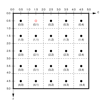
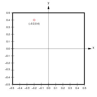
Another subtle distinction between matrices and rasters is that raster data is typically georeferenced; this means that each cell is associated with a specific geographic rectangle on the Earth’s surface with some positive area. That in turn means that each pixel value is associated not only with its pixel/image coordinates but also with the continuous coordinates of every spatial point within that physical rectangle. That is, there is a continuum of spatial coordinates associated with every pixel as opposed to a single pair of pixel coordinates. For instance, in the $5\times5$ grid of pixels shown below in the left plot, the red dot associated with the pixel coordinates $(0,1)$ is located at the center of that pixel. At the same time, the right plot shows a red dot with continuous coordinates $(-0.2,0.4)$.

(from http://ioam.github.io/topographica)

There are two important distinctions to observe:

• Image coordinates are typically expressed in the opposite order of continuous coordinates. That is, for image coordinates $(r,c)$, the vertical position—the row $r$—is the first ordinate and the horizontal position—the column $c$—is the second ordinate. By contrast, when expressing a location in continuous coordinates $(x,y)$, conventionally, the horizontal position $x$ is the first ordinate and the vertical position $y$ is the second ordinate.
• The orientation of the vertical axis is reversed between pixel and continuous coordinates (even though the orientation of the horizontal axis is the same). That is, the row index $r$ increases downwards from the top left corner in pixel coordinates while the vertical continuous coordinate $y$ increases upwards from the bottom left corner.

Conflicting conventions with zero-based indexing and order of coordinates are a source of a lot of programming headaches. For instance, in practical terms, some GIS tools require coordinates to be provided as (longitude, latitude) and others require (latitude,longitude). With luck, GIS users can rely on the software tools to handle these inconsistencies transparently (see, e.g., this discussion in the Holoviz documentation). When computed results don’t make sense, the important point is to always ask:

• which conventions are used to represent raster data as retrieved from any given source; and
• which conventions are required by any GIS tool used to manipulate raster data.

Preserving Metadata¶

Raster data usually has a variety of metadata attached to it. This can include:

• the Coordinate Reference System (CRS): possible representations include the EPSG registry, Well-Known-Text (WKT), etc.
• the NoData value: sentinel value(s) to signal missing/corrupted data (e.g., -1 for integer data or 255 for unsigned 8-bit integer data, etc.).
• the spatial resolution: the area (in suitable units) of each pixel.
• the bounds: this is the extent of the spatial rectangle georeferenced by this raster data.
• the timestamp: when the data was acquired, often specified using Coordinated Universal Time (UTC).

Distinct file formats use varying strategies to attach metadata to a given raster dataset. For instance, NASA OPERA data products typically have filenames like:

OPERA_L3_DIST-ALERT-HLS_T10TEM_20220815T185931Z_20220817T153514Z_S2A_30_v0.1_VEG-ANOM-MAX.tif

This name embeds a UTC timestamp (20220815T185931Z) and an MGRS geographic tile location (10TEM). File-naming conventions like this allow raster data attributes to be determined without retrieving the entire dataset; this can reduce data transfer costs significantly.

Using GeoTIFF¶

There are numerous standard file formats used for sharing many kinds of scientific data (e.g., HDF, Parquet, CSV, etc.). Moreover, there are dozens of specialized file formats available for Geographic Information Systems (GIS) e.g., DRG, NetCDF, USGS DEM, DXF, DWG, SVG, and so on. For this tutorial, we’ll focus exclusively on using the GeoTIFF file format to represent raster data.

GeoTIFF is a public domain metadata standard designed to work within TIFF (Tagged Image File Format)) files. The GeoTIFF format enables georeferencing information to be embedded as geospatial metadata within image files. GIS applications use GeoTIFFs for aerial photography, satellite imagery, and digitized maps. The GeoTIFF data format is described in detail in the OGC GeoTIFF Standard document.

A GeoTIFF file typically includes geographic metadata as embedded tags; these can include raster image metadata such as:

• spatial extent, i.e., the area that the dataset covers;
• the coordinate reference system (CRS) used to store the data;
• spatial resolution, i.e., horizontal and vertical pixel dimensions;
• the number of pixel values in each direction;
• the number of layers in the .tif file;
• ellipsoids and geoids (i.e., estimated models of the Earth’s shape); and
• mathematical rules for map projection to transform data for a three-dimensional space into a two-dimensional display.

As an example, let’s load data from a local GeoTIFF file using the Python rioxarray package.

The rioxarray.open_rasterio function has loaded raster data from the local GeoTIFF file into an Xarray DataArray called da. We can examine the contents of da conveniently in a Jupyter notebook.

This raster is fairly high resolution raster ($3600\times3600$ pixels). Let’s take a smaller slice (i.e., sampling every 200th pixel) by instantiating the Python slice object subset and using the Xarray DataArray.isel method to construct a lower resolution array (that will render faster). We can then make a plot (rendered by Matplotlib by default).

Observe that the plot is labelled using the continuous (easting, northing) coordinates associated with the spatial extent of this raster. That is, the subtle book-keeping required to keep track of pixel and continuous coordinates has been handled transparently by the data structure’s API. This is a good thing!